Due to the utilization of coastal and offshore spaces and the need for designing structures on coastal areas, important external forces must be considered, including wave information such as wave heights, wave periods, and wave directions. It is essential to know these wave parameters in many coastal engineering applications for the protection and restoration of the nearshore environments such as beaches and natural habitats.

With newly developed technologies, the hardware specifications for wave gauges are being upgraded. Especially, nautical radar wave gauges have improved their accuracy due to improved hardware and software performances. Alpers and Hasselmann (1982) introduced an estimation of significant wave heights by regression of energy spectra using SAR (Synthetic Aperture Radar). Instead of SAR, Young et al. (1985) were the first to utilize X-band nautical radar for estimating significant wave heights. There have been many studies for improving the performance of wave gauges using X-band marine radar (nautical radar). However, the accuracy of wave heights measured by X-band radar is relatively low compared to other wave gauges. Therefore, further research is needed to improve the accuracy of X-band marine radar.

Wave gauges have two categories of methods for measuring waves. Point measuring type of wave gauge is waverider buoys, P-u-v (pressure and u-v velocity) gauge and ADCP (acoustic doppler current profiler), etc. Measuring waves over a sea surface area can be done with a radar. Buoys, P-u-v gauges, and ADCP measure wave surface elevations directly at sea, while radio detecting and ranging (radar) measures waves through remote sensing using microwaves. The results from each wave gauge are not the same but similar because the steady-state sea has ergodicity. Ergodicity means that the distribution in one place over time has the same behavior as the spatial distribution in a fleeting moment. Therefore, wave information obtained from the point measurement and the area measurement is assumed to be the same under steady ergodic condition.

Table 1 shows the characteristics of wave gauges. Waverider buoy, P-u-v gauge and, ADCP have high accuracy compared to radar and initial installation costs are lower than that of radar system. Even though radar wave gauge has a low accuracy in wave height measurement but has many advantages. Radar wave gauge has low life cycle cost not only because the durability is very high but also because maintenance costs are very low compared to other wave gauges. Additionally, as radar can measure waves remotely depending on the distance from the radar system, it can measure waves without any limitations of water depth including very shallow water depth such as surf zone as well as deep water. Importantly, radar can measure waves together with sea surface current velocity and wave number spectrum. Radar can also obtain wave information directly in real time.

The received radar signal is not the direct information about the actual height of the wave, but the distribution of the energy intensity received by the radar signal scattered by the waves. Therefore, it is necessary to estimate the measured radar signal to get wave information correctly. Alpers and Hasselmann (1982) presented the algorithm for calculating the signal to noise ratio from SAR images to estimate significant wave heights. Nieto et al. (2004) showed the detail of the algorithm and introduce MTF (Modulation Transfer Function) to estimate significant wave heights from the X-band marine radar deployed in the field.

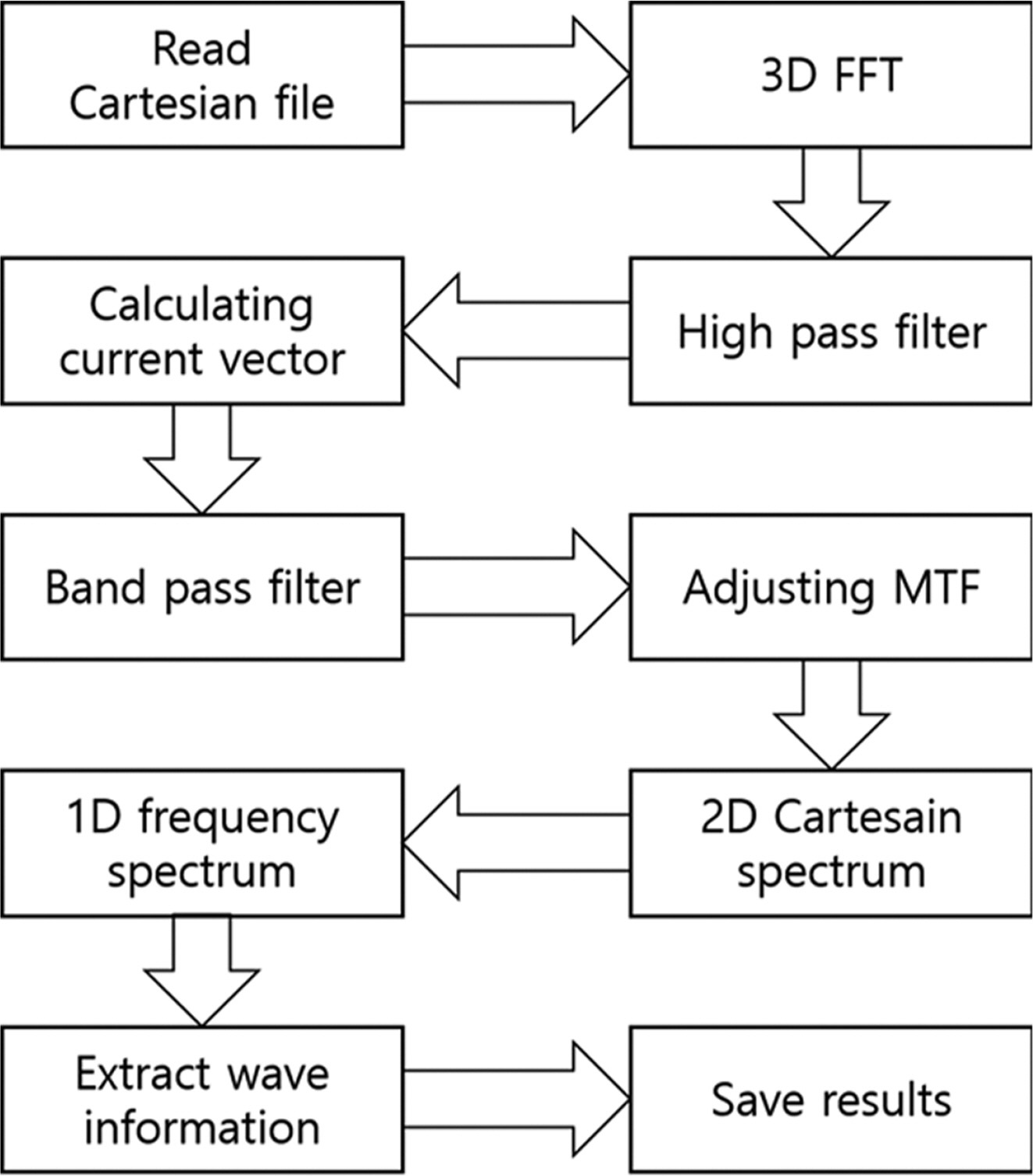
Fig. 1 shows the process of estimating wave information. Time series of sea surface images in the form of Cartesian coordinates are analyzed to get 3 dimensional image spectrum through 3D fast Fourier transform (3D FFT). Then, the current vector is calculated after high pass filtering. By applying the pass band filter based on the wave dispersion equation, we can obtain the 3D wave spectrum. Integration of the 3D wave spectrum over frequency yields the 2 dimensional wave number spectrum. Applying proper MTF, we can obtain wave number spectrum. We can also derive the wave frequency spectrum as well as directional wave frequency spectrum by the transformation of coordinates. From the wave frequency and directional frequency spectrum, we can extract wave information such as significant wave heights, peak period, and mean wave direction, etc.

The major signal components of the radar system are the target, clutter, and noise. In a general case, the radar has a target, such as a ship or an airplane. However, X-band radar wave gauge systems use sea clutter for analyzing wave parameters such as the significant wave height and peak period. Alpers and Hasselmann (1982) defined the sea clutter as the ‘signal’, other clutter as ‘clutter’and noise as ‘thermal noise’.

Alpers and Hasselmann (1982) estimated significant wave heights with synthetic aperture radars by separating the wave signal from background noise, so-called ‘signal to noise ratio’ (SNR). The SNR can be used to determine significant wave heights with linear regression as in Eq. (1).

The SNR is determined by separating the spectral components using the dispersion relation. Nieto (2000) represents the SNR as follows:

where F⁽³⁾(k_x, k_y, ω) is the power spectral density filtered by the dispersion relation, Fbgn(3)(k_x, k_y, ω) is the power spectral density outside the dispersion relation.

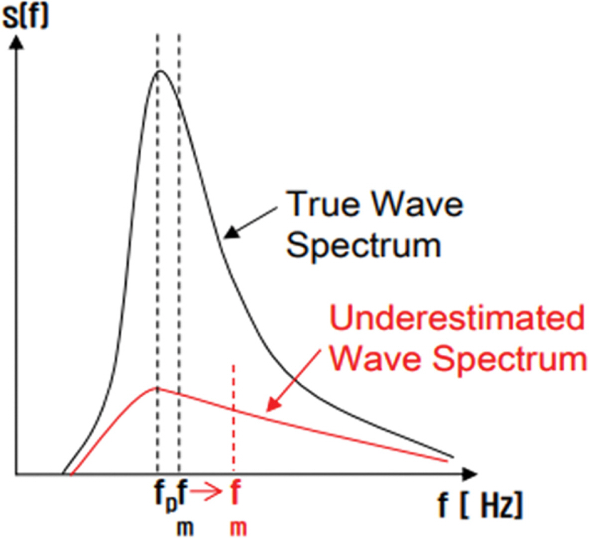
The estimation of significant wave heights using SNR and peak period has been proposed by Ahn et al. (2014) and Ahn et al. (2015). A case with low energy reception due to low energy backscattering of smooth surface waves is considered to significantly underestimate the significant wave height. It is because of the absence of ripples that are generated by local wind. Smooth sea surfaces of swell waves without ripples mean no Bragg resonance occurred and result in weak backscattered signals. As a result, the radar signal is not enough for an analysis of wave heights by using SNR only. Fig. 2 shows the underestimated frequency spectrum of low energy reception case such as smooth surface swell waves. However, the peak frequency of an underestimated wave spectrum is usually identical to the true wave spectrum of swells. On the other hand, the mean frequency of the observed energy spectrum is usually higher than the mean frequency of the true spectrum. Therefore, proper calibration of significant wave heights could be achieved by including peak frequency information.

ANN (artificial neural network) is a method of finding the output of each neuron by some nonlinear function of the sum of its inputs. In nature, each piece of data has no exact linear regression. Although there are multiple methods of regressions, it is difficult to generalize expressions for a formalized regression in the case of a complex model. ANN can help solve this problem.

The input data for a neural network includes the connections between neurons. After processing input data, the networks produce their output data. Comparing between the output data and target data, the network adjusts its own weighting. This process continues until the satisfying conditions, such as the error, are lower than a specific constant or the number of iterations exceeds a specific constant. The structure of a neuron is expressed in various ways depending on the type of input and neuron.

The ANN process consists of two parts. The first is training the data and the second is simulating the data. In the training part, the dataset is preprocessed as input variables. Next, the ANN network is created, which is a feedforward backpropagation network with a tangent-sigmoid transfer function in a hidden layer and a linear transfer function in the output layer. By using the data and the network, the network is trained for estimating the target value. After the training, the output weights, bias, and other conditions are saved from the trained network. The next part is to simulate a dataset using the trained network.

We compared the results of different estimation methods applied to the data obtained at Hujeong Beach, Uljin which is located on the east coast of the Korea peninsula

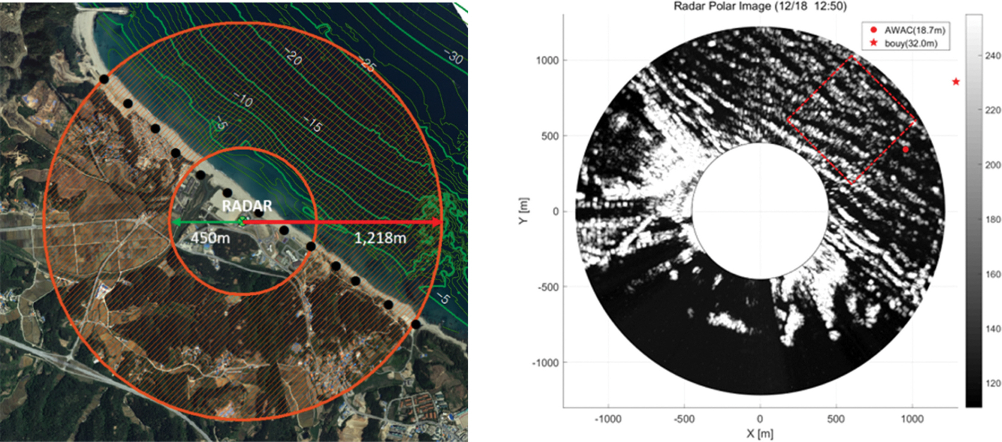
The radar was stationed at a height of 20 m above sea level and scanned sea surfaces of radius from 450 m to 1,218 m as is shown in Fig. 3. The shoreline of Hujeong Beach stretches from the northwest to the southeast. Therefore, waves coming from the northeast are frequently observed. The data used for the analysis had been obtained from December 15 to December 23, 2014. In every 20 minutes, the radar, which was rotating at 24 rpm, acquired 32 polar images and the time interval of each image is 2.5 seconds. The radar was rotating for 80 seconds in every 20 minutes.

Fig. 3 shows a polar radar image obtained at 12:50 pm on December 18, 2014. In the figure, the red circle is the location of the Acoustic Wave and Current Profiler (AWAC) of Nortek deployed at water depth of 18.7 m and the red star represents a waverider buoy deployed at water depth of 32.0 m. The red dotted rectangle in the figure is a Cartesian image used for estimating significant wave heights and other wave parameters. The center of the Cartesian image is 850 m away from the radar with dimensions of 600 m × 600 m.

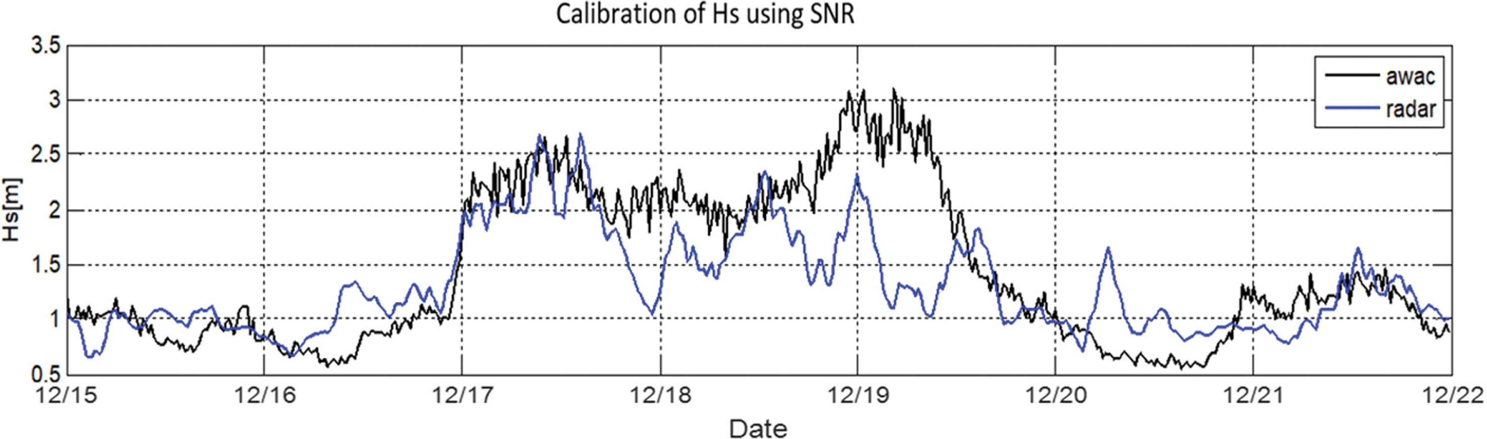
Fig. 4 shows time series of significant wave heights estimated by SNR during winter storm. From 12/17 22:00 to 12/19 12:00, the estimated significant wave heights from the radar are significantly underestimated after 20/18 18:00. This is because of the absence of ripples due to weak local wind velocity, which affects weak Bragg resonance condition.

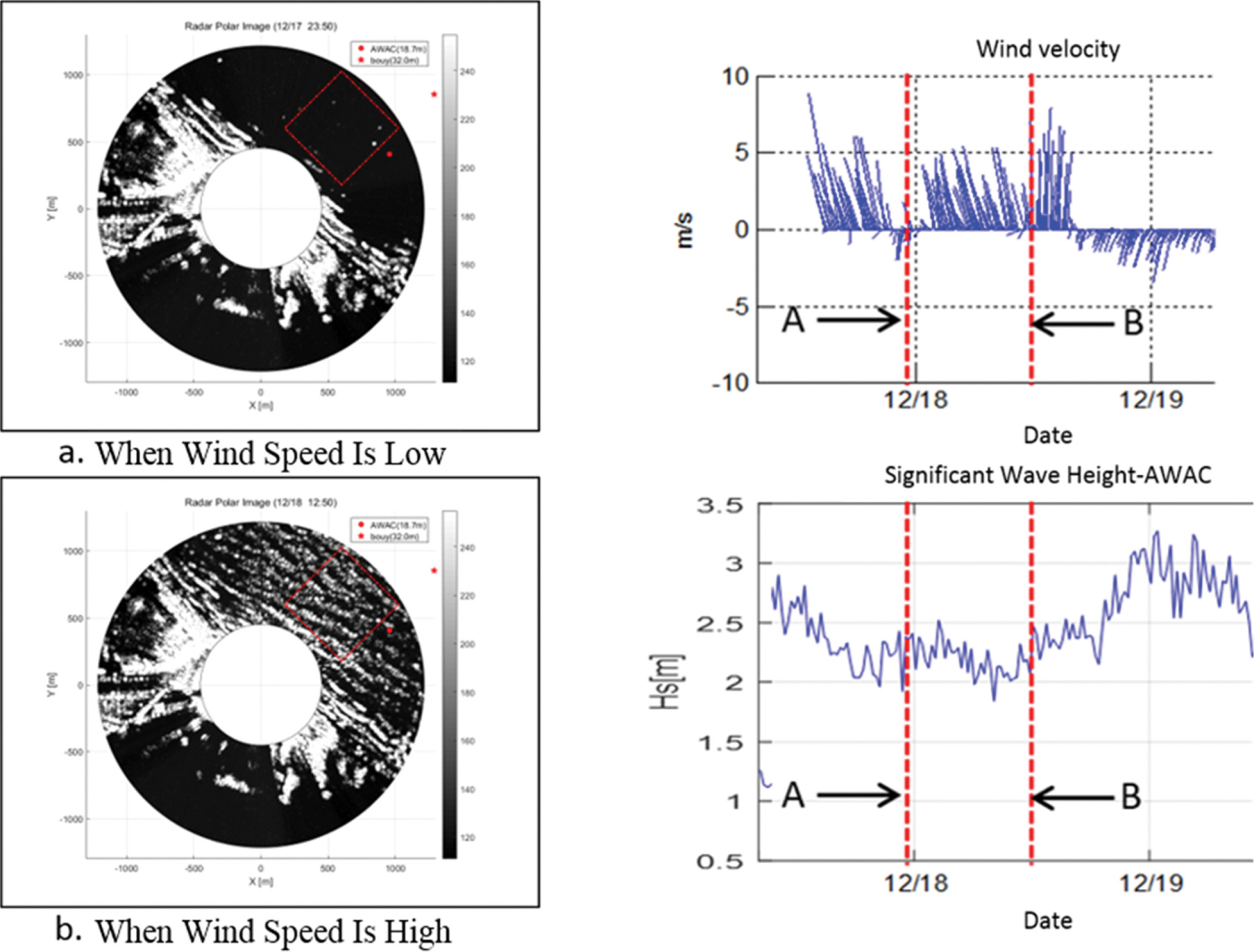
Fig. 5 shows polar radar images during the storm in 2017. Both polar images in the figure have similar significant wave heights of 2.28 m and 2.03 m according to AWAC measurement, but radar images have very different sea surface undulations and estimated significant wave heights of 1.05 m and 2.15 m, respectively. The reason for this discrepancy is that local wind is not blowing enough to make ripples on the surface of the waves and thereby cause weak backscattering of signals at the time of measurement. Wind information, including not only the speed but also direction, is important for backscattering to occur. As shown in the figure, red dot lines A and B drawn in wind velocity stick and significant wave heights estimated from radar images are 1.05 m and 2.15 m, respectively. Red dot line A is the case where the wind direction is from land to sea and wind speed is very weak. However, Red dot line B is the case where the wind direction is from sea to land and wind speed is high enough to make ripples for Bragg resonance to occur.

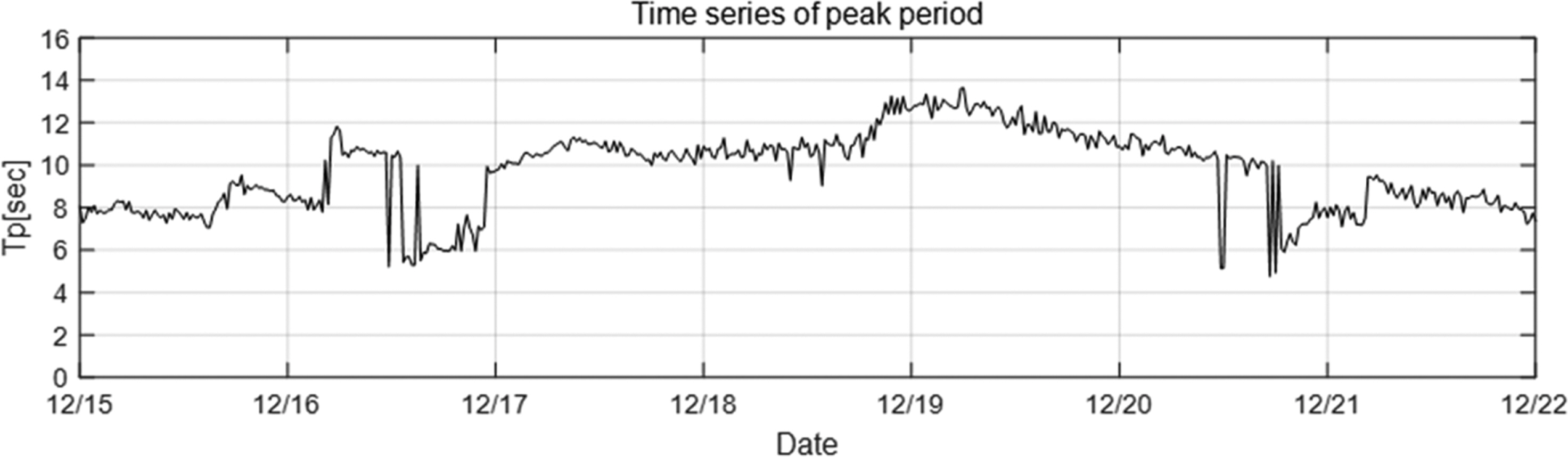
Fig. 6 shows the time series of peak periods (Tp) obtained from the AWAC. As is shown in the figure, peak periods are greater than 10 sec from the beginning of winter storm and maintained its period even after the storm. During the storm, wave heights are varying but the variation of peak periods is relatively small. It is because wave periods are considered to be influenced by the wave travelling distance but not by local wind. Wind waves are caused by local wind, but swell waves are propagated from distant seas. Therefore, a swell is related neither to the local wind speed nor to the wind direction. In order to calibrate wave heights from radar images which are influenced by local wind speed and direction, it may be good to use peak periods to compensate for the underestimated significant wave heights.

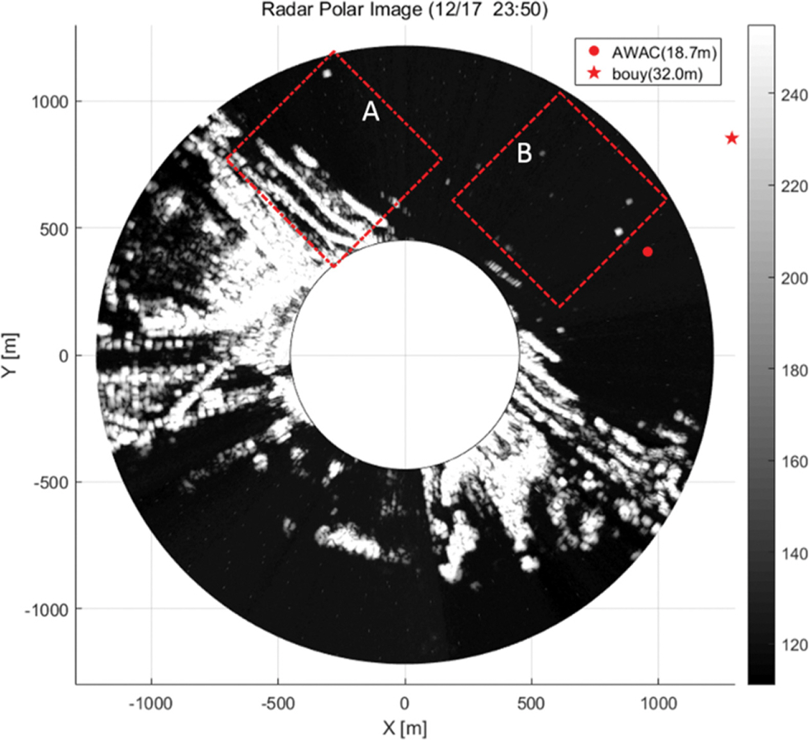
To use the peak period data, catching the peak periods accurately is important in radar images. Fig. 7 shows the radar polar image obtained at 2014/12/17 23:50. The red dotted rectangular ‘B’ area is the target Cartesian region to calculate wave parameters from the radar. In this area, the Cartesian image does not show enough radar signal to obtain the wave information. However, the radar image in the ‘A’ area where breaking waves occurred near the coastline, is an adequate place to obtain wave peak period. As far as nonlinear interactions of wave frequency components are not dominant, peak wave periods are identical in regions A and B. Therefore, we programmed to choose the region whenever we need to obtain necessary wave parameters such as wave period.

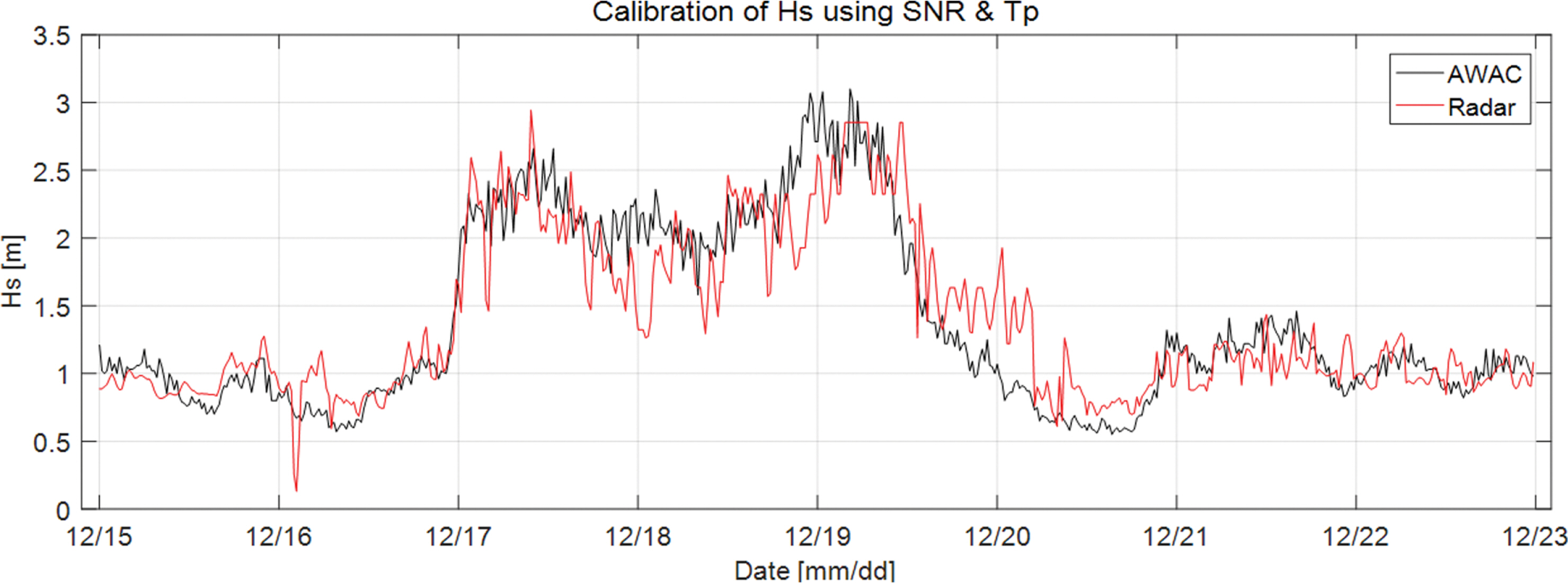
Fig. 8 show a comparison of significant wave heights from the AWAC and those estimated from radar by considering SNR and T_P. These results have a RMSE (root mean square error) of 0.29 m, a maximum error of 0.99 m and an R² (coefficient of Determination) of 0.79. These results are more accurate than those estimated using SNR only as is shown in Fig. 4.

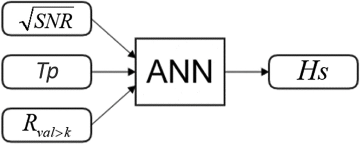
Estimation using an ANN is used for improving the accuracy of estimating significant wave heights. Fig. 9 shows the structure of the ANN to make the feedforward backpropagation network. The input vector uses the parameters SNR, T_P and R_val/k.

Parameter R_val/k is used to represent wind condition which is defined as

where N_u is the number of pixels higher than the k value in the target image. N_t is the number of pixels in the target image.

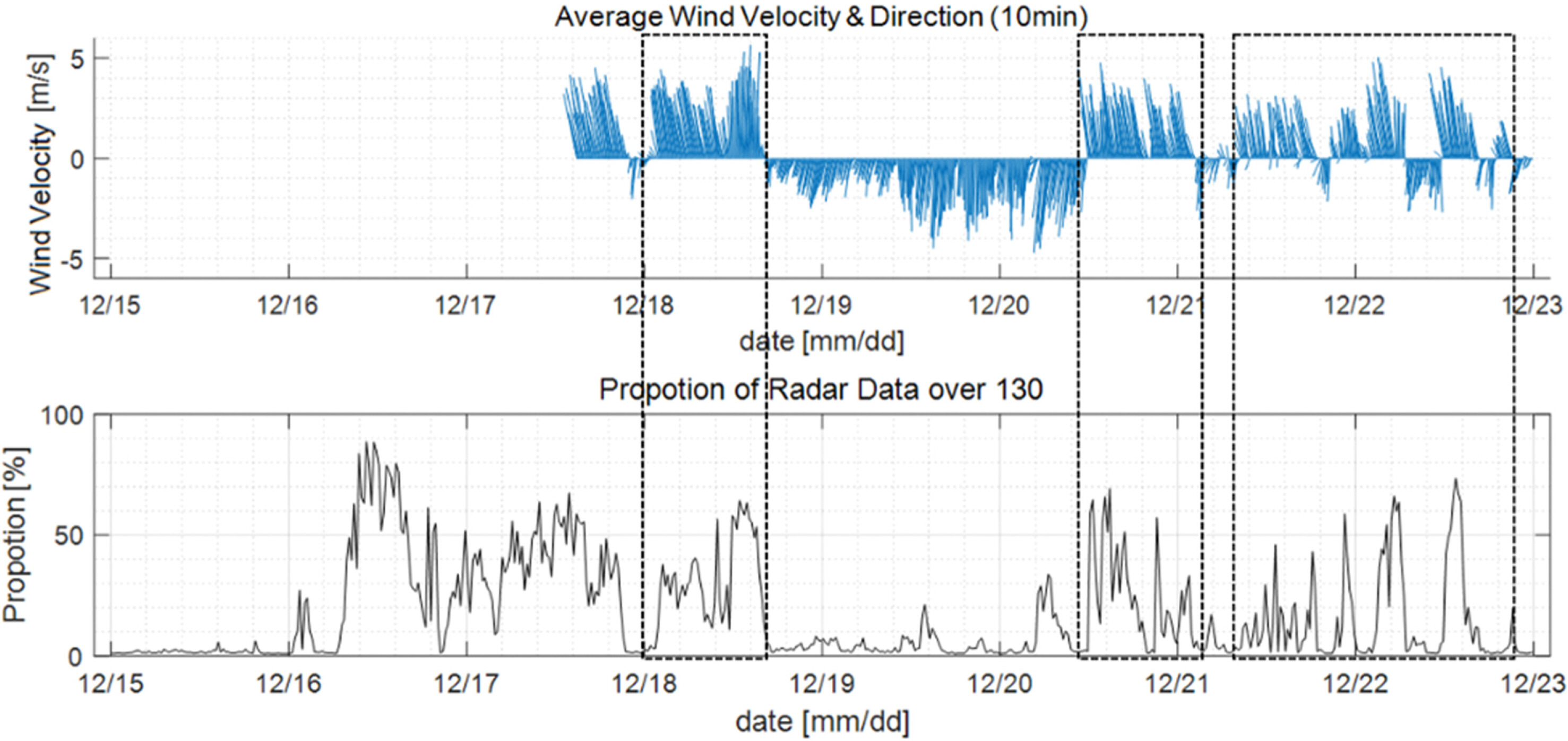
Fig. 10 shows the variation of R_val/k which is almost zero when there are not much ripples on the sea surface. This condition occurs when the wind is blowing from land to sea direction or no local wind exists.

The ANN used for Hs learning consists of an input layer, a hidden layer, and an output layer. In this study, The number of neurons in the hidden layer was 10. Levenberg-Marquardt was used for the ANN learning method, and the tangent-sigmoid function was used for the transfer function. The total number of radar data used in the analysis is 576. The number of ANN training dataset is 144 which is uniformly sampled from total data. In the training, 70% of the training data was used for training, 15% for verification and the remaining 15% for testing, and it was randomly sampled.

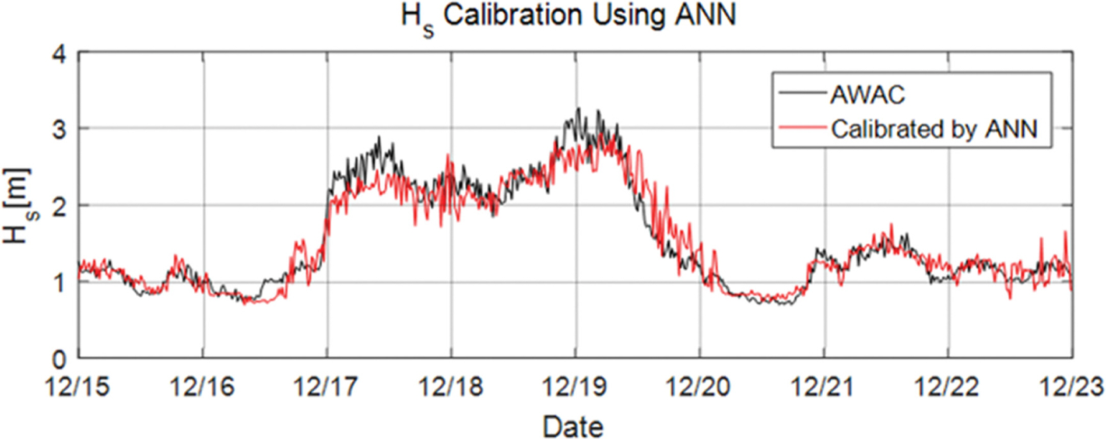
Fig. 11 shows the results of the estimated significant wave heights using ANN compared with those obtained from AWAC. These results have an RMSE of 0.22 m, a maximum error of 0.80 m and R² of 0.89. The RMSE and the maximum error of the results using ANN is improved by 0.07 m and 0.19 m, respectively, compared to the result obtained using SNR, T_P. R² is also increased by 0.10.