


1. Introduction
Relations between wave pressure and free surface elevations have been applied to field measurements since 1947, when Folsom (1986) and Seiwall (1947) used pressure gauge to measure free surface elevations. Since then, a number of methods to obtain free-surface elevations from wave pressures have appeared whereas almost no interest was shown in modelling wave pressures on the basis of free-surface elevation. This obviously results from the fact, that it is usually easier to measure wave pressure than surface elevation. However, in some cases, such as apparatus failure, a possibility for obtaining wave pressures from the free-surface records might be useful. Also, in some maritime engineering applications, measuring pressure is more difficult than recording free-surface elevations. For example, it is possible to collect in a relatively easy way accurate measurements of water surface elevations using remote sensing techniques with a down-looking laser device installed on an offshore platform. In such situations it is sufficient to install underwater measuring equipment for a limited period of time only, allowing model construction and estimation of its parameters. Then, measured time series of free-surface elevations may be used to provide the wave pressure data via the model developed.
Most of the procedures transforming wave pressure series into surface elevations time series can be modified to apply them in the reverse direction. These methods can either work globally (processing entire series at a time) or locally (small part of a series is processed). Global methods include:
- Linear Transfer Function (LTF) as summarized by Bishop and Donelan (1987), Tsai and Young (2001), Grace (1970);
- Nonlinear modification to LTF developed by Hashimoto et al. (1997) on the basis of Tick’s paper (1959);
- Empirical Transfer Functions presented by Kou and Chiu (1994). The following local methods have been recently developed:
- Local Sinusoid Approximations (LSA) and empirical LSA methods by Nielsen (1989);
- Local Polynomial Approximations method (LPA) developed by Fenton (1986) and simple LPA by Fenton and Christian (1989);
- Local Fourier Approximations (LFA) presented by Sobey (1992), Barker and Sobey (1996 and 1997).
Linear Transfer Function (LTF) method is a simple derivation from linear wave theory: Fourier transform of freesurface elevation  is multiplied by transfer function L(f), then transformed back to time domain and finally scaled by gravity and water density ρg. L(f) takes the familiar form of L(f;a, h) = cosh[k(f)·(z + h)] ⁄ cosh[k(f)·h] with the wave number k related to the frequency f via dispersion relation, vertical coordination z and mean water depth h. This method is still the most frequently used one despite its inaccuracy shown by Hom-ma et al. (1966), Grace (1970), Cavaleri (1980), Bisel (1982), Lee and Wang (1984), Wang et al. (1986) as well as authors using local methods listed above.
is multiplied by transfer function L(f), then transformed back to time domain and finally scaled by gravity and water density ρg. L(f) takes the familiar form of L(f;a, h) = cosh[k(f)·(z + h)] ⁄ cosh[k(f)·h] with the wave number k related to the frequency f via dispersion relation, vertical coordination z and mean water depth h. This method is still the most frequently used one despite its inaccuracy shown by Hom-ma et al. (1966), Grace (1970), Cavaleri (1980), Bisel (1982), Lee and Wang (1984), Wang et al. (1986) as well as authors using local methods listed above.The method is generally recognized as working well in laboratory tests for linear waves, especially when the pressure gauge is installed at relatively high z-elevation (Bisel, 1982; Bishop and Donelan, 1987; Tsai et al., 2005). For nonlinear waves, LTF method fails to model high and low frequency behavior of processed series. Partially this results from cutting theoretical transfer function at some frequency fc by setting its values to 0 for frequencies fc and higher. Otherwise the infinitely increasing LTF multiplied by the pressure spectra would produce false values in high frequency region of the simulated free-surface elevation spectra. Therefore, the linear transfer function is truncated, which results in producing surface elevation series with no energy contained at frequencies fc and higher (Lee and Wang, 1984). Moreover, LTF is commonly multiplied by an empirical constant whose value seems to depend on location. Review of values can be found in Grace (1970) as well as in Bishop and Donelan (1987). Further empirical LTF developments by Kuo and Chiu (1994) clearly oversimplify the transfer function, replacing water depth and gauge depth dependency with a single empirical modification. That resulted in overestimating wave heights by as far 30% during a field experiment reported in (Tsai et al., 2005).
Linear Transfer Function method can be corrected in high frequency region as suggested by Hashimoto et al. (1997) by setting LTF values for frequencies higher than fc equal to a constant value referring to fc. Hashimoto et al. (1997) proposed a new method to determine fc based upon analytical properties of expressions for weakly nonlinear, second order spectra given by Tick (1959).
Local methods start with fitting sine curve (LSA), complex polynomial (LPA) or Fourier series (LFA) to a portion of pressure series surrounding the time of interest. Consequently, nonlinear dynamical equations are solved to find potential function and free surface elevation. Details can be found in: Nielsen (1989), Fenton (1986), Fenton and Christian (1989), Sobey (1992), as well as in Barker and Sobey (1996 and 1997). Detailed comparison made by Townsend and Fenton (1996) showed that LPA work generally better than global methods (LTF) with regular waves and in cases when pressure gauge was set at greater depths. However, in a case of random waves LPA performed similarly to LTF due to higher noise-to-signal ratio. As Townsend and Fenton (1996) used only water tank generated data, LPA performance in field conditions remains unknown. Since fitting a polynomial to a signal is sensible to high noise-tosignal ratio, the procedure might perform not so well in transforming elevations to pressures. This might result from fitting a complex polynomial to a more noisy free surface elevation series. LSA, in turn, was found by Townsend and Fenton (1996) more robust against the noise. However, a disadvantage of the LSA methods is the failure just above the trough of the wave (Townsend and Fenton, 1996).
In this study we apply System Identification (SI) techniques to develop models transforming free-surface elevations into wave pressures. In general, SI is concerned with constructing dynamic models of a system in which variables of different kinds interact and produce observable signals that are called outputs and which are of interest to us. The system is simulated by external signals that are called inputs. We say the system and its components are dynamic when the current output values depend not only on the current input but also on their earlier values.
In the presented paper we suggest that it is possible to create two linear time invariant dynamic models linking the free-surface elevation and wave pressure series: one allowing for wave pressure simulation using free-surface elevation as an input variable and second for free-surface elevation simulation using wave pressure as input data.
Obviously, on shallow water such a SI model is valid only for a given location, mean water level and-the most important-for a constant distance between the mean water level and pressure transducer depth. Furthermore, a linear model estimated in time domain using narrow-banded data will be most reliable when applied to input data with most of the spectral energy located close to the spectral band of estimation data. As the spectral density distribution S(f) over the frequency f can be roughly characterized by the mean energy wave period TE = [∫f–1S(f)df] ⁄ [∫S(f)df] it might be feasible to the combine spectral information with the pressure transducer depth z and the water depth using the value of linear transfer function LE taken at fE = TE–1, i.e. LE = L(fE;z, h). The use of a simple rescaling coefficient based upon LE might increase the reliability of simulation in case when the spectral properties of input data differ from the properties of estimation data.
In consequence, presented SI models can be applied to replace data occasionally disturbed due to equipment failure or conservation or to monitor data consistency in real time. Further research is being directed to extend the models onto wider transducer depth range and provide better simulation in case of input with spectra located outside the original band of estimation data.
System Identification techniques have been successfully applied, among others, to model wave velocities and accelerations based on free-surface records by Cieoelikiewicz and Gudmestad (2001 and 202) as well as to Morrison equation improvement by Stansby et al. (1992), Selvam et al. (2001). Moreover, nonlinear System Identification methods are a typical tool in marine engineering applications such as ship dynamics (Bendat, 1997; Faltisen, 1990; Mulk, 1994) or structure modelling (Bhattachararyya et al., 2001).
This paper extends results presented in previous studies (Cieoelikiewicz and Gudmestad ,2001 and 2002) by application of SI methods to either free-surface elevation or wave pressure simulation and rescaling model results to use in case of slightly different (within 1 m range) pressure gauge depth, water depth and different sea state as manifested by mean energy wave period TE differing from 3.9 to 5.6 s and significant wave height from 0.9 to 1.7 m in Table 1.
Table 1.
Free-surface elevation record #, mean energy wave period TE, peak wave period Tp, wave length λTE associated with TE, linear transfer function value LE, significant wave height Hm0, pressure transducer depth z and mean water depth h.
2. System Identification Procedures
This section briefly presents the framework of traditional System Identification techniques, which will be used in various applications: model structure and input/output data will be changed. In particular, the wave pressure simulation model will use transformed series of free-surface elevation as an input and free-surface elevation model will use transformed wave- pressure as an input.
Let Y(t) denotes the output data sequence of the system, i.e., pressure record pt in case of wave pressure simulation. The input data vectors Qt of NQ dimension are composed of the free-surface elevation sequence ζ(t).We include the random disturbance as an additive filtered white noise. We assume in this study that the wave system can be described by a linear time-invariant model which is specified by the sequence of impulse response series gq(k), q = 1, ..., NQ and the weighting function h(k) of the random additive disturbance, k = 0, 1,…,∞, and, possibly, the probability density function of the white-noise εt. It is worth noting, that despite the assumption of a linear model we are still able to incorporate in a system the nonlinearities that have the character of a static nonlinearity at the input side, while the dynamics of the system itself is linear. In case the nonlinearity is known, say as a function F, a certain input variable U(t) can be transformed into Q(t) = F{U(t)} and the system can be treated as linear. We will have such a situation in this study. A complete model is given by the following relationship (Ljung, 1987; S derstr m and Stoica, 1989):

in which f is the forward shift operator defined by fQ(t) = Q(t + 1), G is the transfer function of the system and G(f)Q(t) is short for  Gq(f)Qq (t) and for any q = 1, 2, …, NQ
Gq(f)Qq (t) and for any q = 1, 2, …, NQ
As mentioned above, we assume that the disturbance N can be described as filtered white-noise, so

where
Within SI we work with structures that permit the specification of G and H in terms of a finite number of numerical values. As is common, we assume that ε(t) is Gaussian, in which case the PDF is specified by the first and second moments. Thus, a particular model (1) is entirely determined in terms of a number of numerical coefficients which are included as parameters to be determined. The purpose of SI is to determine the values of those parameters. If we denote the parameters in question by the vector θ, and if we take into account the relation (4), the basic description of the modelled system becomes
which is a set of models, each of them associated with a parameter value θ.
A commonly used way of parameterizing Gq and H is to represent them as rational functions of f−1 and specify the numerator and denominator coefficient in some way (Ljung, 1987). Such model structures, which are known as black-box models, were utilized in this study. A few different model structures were tested. In this paper the examples demonstrating the results of SI with one of the simplest model structures, i.e., autoregressive with extra input (ARX) model structures for wave pressure will be presented. For the ARX model in multiinput single-output version equation (6) may be rewritten as

where A(f)Y(t) is the autoregressive part while B(f)Q(t) is the extra input of the ARX model in which

and for q = 1, 2, …, NQ
The vectorial parameter θ to be determined is in this case composed of coefficients of the polynomials A and Bq
where NA, NB1, NB2, …, NBNQ are the orders of the multi-input single-output ARX model.
In the present study the models were estimated using least-squares methods. If we denote by N the length of the time series Y(t) and write
where tmin = max{NA, NB1, NB2, …, NBNQ}, then the least-squares estimate of the parameter vector θ* is defined as

here arg[·] means “the minimizing argument of the function.”
3. The experiment
The available data were collected on February 12 and March 10~11, 1976 at oceanographic tower Aqua Alta of CNR located in the northern Adriatic Sea approximately 7 Nm off the coast of Venice at 16 m water depth. Tower construction, equipment and prevailing hydro-meteorological conditions were described in great detail by Cavaleri (1973, 1979, and 1999) and also by Cavaleri and Zeccheto (1987). Very light structure and instruments location at the vertical of an additional platform allowed to avoid any significant structure influence on measured quantities. The instruments were attached to a cart sliding on two vertical wires with a rotating arm, which enables their alignment in the optimal direction. The accuracy of cart positioning was very high as the length of wires was known within a centimeter and lateral deflection did not exceed a few centimeters.
Free surface elevation were recorded using resistance wave staff developed at CNR, calibrated under ‘wet conditions’ taking into account splashing and suction effects (Cavaleri, 1973). Overall wave staff error was estimated not to exceed 2.5%.
Both pressure and free surface elevation were recorded with sampling interval 0.25 s and four digit accuracy on magnetic tape. During the experiment the cart was lowered to depths of approximately 2, 4, 6, 8 and 10 m recording each time signal lasting for some 30 minutes. All the wave pressure time series were scaled down by the water density and the gravity factor ρg and are expressed in [m].
For estimation of both free-surface and wave pressure models, record #38 was chosen together with 9 other records for validation. These validation data were recorded at similar pressure gauge depth and similar water depth as presented in Table 1. Various wave conditions are represented by these records with the mean energy wave period TE ranging from 3.95 to 5.63 s (corresponding to wave length λTE from 24 to 48 m), peak period Tp ranging from 4.8 to 6.57 s and the significant wave height Hm0 from 0.9 to 1.86 m.
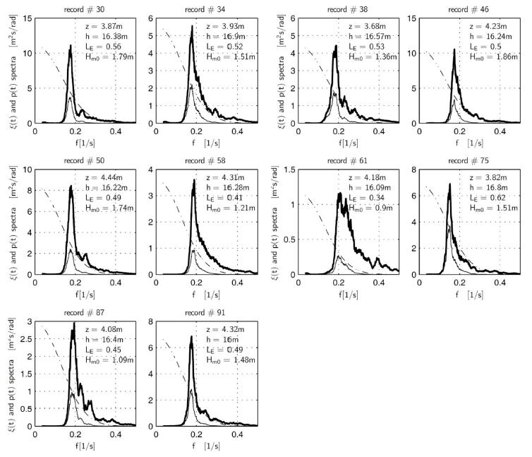
The compound effect of various wave conditions (manifested with various free surface elevation spectra in Fig. 1) and slightly varying z and h can be summarized with the value of LE being the linear transfer function value at the frequency TE–1, the pressure gauge depth z and the water depth h . Obviously, as a single linear model can not be expected to cover that range of wave conditions as well as pressure and water depth variability, as caling factor based on LE value will be used to improve accuracy of simulation. To show the variations in wave conditions in greater detail, free-surface elevation and pressure spectra are presented in Fig. 1 together with linear transfer function L(f) which might be interpreted as the first approximation to frequency response of the system. Note, that although usually L(f)∈[0, 1], the L(f) curves in Fig. 1 are scaled up by a maximum value of ξ(t) spectrum to show how the peak energy of the ξ(t) is transformed into p(t).
4. Application of SI techniques
In this section, techniques presented in section 2 are used to construct two distinct models: one referred to as free-surface model for simulating free-surface elevation using wave pressure as an input whereas the second one, referred to as wave pressure model will use free-surface elevation to simulate wave pressure. Despite working in opposite direction both pressure and free-surface models share the same structure of ARX model presented in (7)~(9) with single output, multiple inputs and A = 1. The A operator polynomial is reduced to identity expressing the fact that y(t) at time t does not depend on its previous values but depends {y(tp), tp<t} on past and present values of input Q(t). As both models share also the structure of input vector Q(t), they will be presented jointly.
Data preprocessing included standard quality check procedures and high-frequency noise removal eliminating frequencies higher than 0.7 Hz (periods shorter than 1.3 s) using Butterworth anti-causal filter. The low-frequency part of records, which form an additional input in the sys- tem identification technique described below, is defined as containing frequencies lower 0.03 Hz (periods longer than 30 s).
As stated in section 2, for efficient model estimation, the choice of model orders, time delays and input vectors is crucial. Delays of both models were set to zero due to reported fast instruments response and the nature of modelled system. Polynomial A was set to identity to provide greater stability with no loss on modelling accuracy comparing to, for example, models with NA = 10, which might be attributed to the high correlation between input an dout put of the system.
Construction of input vector and model orders, in turn, resulted from an iterative search for the best wave pressure model with sample data containing one elevation-pressure set and various input structures considered. Best results were achieved with an input vector consisting of free-surface elevation ξ(t),its square ξ(t)2 and low frequency component ξL(t) that is: Q(t) = [ξ(t), ξ(t)2, ξL(t)]. The free-surface elevation square proved to be especially useful incase of wave kinematics (Cielikiewicz and Gudmestad, 2001 and 2002) whereas the low frequency component was found to improve the performance of pressure models provided model rank in ξ(t) was sufficiently high. The input structure determined during the tests was used in both models. Furthermore, the test indicated that a dedicated model emphasizing the low frequency behavior might be useful. Obviously, when estimation and validation data are distinct parts of the same series (i.e. p(t) and ξ(t) are divided into two separate estimation and validation parts), the simulation results on validation input are better than those achieved with the linear transfer function (LTF) method.
4.1. General model structure
In this paper, an estimated pressure or free-surface elevation model is supposed to perform for similar values of z, h, and wave conditions with possible improvement achieved by simple rescaling of simulated time series. Taking into account the previously reported importance of low-frequency component, both the free-surface elevation and the pressure models will consist of two separate models: one for medium-frequency range GM and another for low-frequency range GL to form model output Y(t) as a sum:

Both GM and GL were estimated independently with:
where u(t) = ξ(t), uL(t) = ξL(t) and tM = pM(t) in case of wave pressure model and u(t) = p(t), uL(t) = pL(t) and yM = ξM(t) in case of free-surface elevation model. Note, that because of low frequency separation, data with ·M subscript contain no low frequency component as it is modelled using its own model GL. The ·L subscript denotes low-frequency part of the series. All models share the same structure of an autoregressive model with extra input (ARX) outlined in (7)~(9) with model orders NA = 1, NB = [80, 80, 80] for main models GM and NA = 1, NB = [80] for the low frequency models GL.
As observed in Fig. 1, linear transfer function L(f) describes the amount of ξ(t) spectral energy transferred to pressure time series p(t) as predicted by linear theory. As the ARX coefficients are determined using narrow-band wave and pressure data, an ARX model, as applied in this study, is not likely to transfer reliably another free-surface elevation into pressure series if its spectrum is far from the spectral band of original data used to estimate the model. It was found that a simple linear scaling of modelled pressure by a ratio of transfer function values LE for energy wave period improved results for almost all simulated pressure time series. The coefficient to multiply ith simulated pressure time series takes the form of:
where index ·e refers to record used for estimation. It is not clear whether scaling should be done using mean energy wave period TE, peak wave period or mean wave period Tm01, but improvements over simulated p(t) were good enough in case of TE. Unfortunately, for free-surface model, an equally good coefficient could not be found easily.
Wave pressure and free surface elevation models were estimated using the free surface elevation and pressure record #38 and validated against the records 30, 34, 46, 50, 58, 61, 75, 87, 91. All pressure data except for the last two records come from the upper pressure transducer as described in section 3 and refer to the roughly the same transducer depth which is around 4 m in water depth of 16.0~16.8 m. No significant improvement was achieved by including any other pressure-elevation set into estimation data.
5. Results
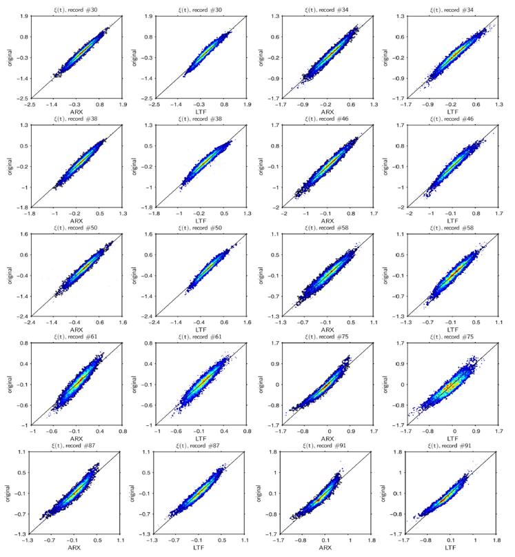
As previously stated, both free-surface and wave pressure ARX models were validated using data collected under slightly different wave conditions manifested in record description in Table 1 and with varying spectra in Fig. 1. Simulation quality was measured using the scatter index εs between simulated and original data for both ARX and LTF methods and by examination of the standard deviation, skewness and kurtosis with values listed in Tables 2 and 3. All the simulated time series were visually compared to original time series using scatterplots shown in Fig. 3 and 5.
Table 2.
Statistics of free-surface simulation using ARX and LTF compared with original data. Record # 38 (in bold) used for estimation

5.1 Free-surface elevation simulation based on time series
Free-surface simulation assumed the ARX model structure outlined in (7)~(9) and input signal structures defined in (14)~(15) with yM and yL in (14) interpreted as a mediumand low-frequency components of free-surface elevation time series.
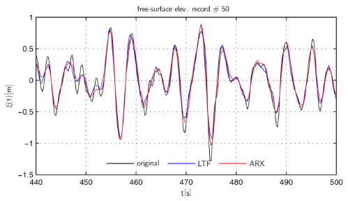
A sample of free-surface elevation time series for the record #50 simulated with ARX and LTF is presented in Fig. 2. For this exemplary sample, the ARX simulation quality is slightly better than LTF. Generally, the quality of free-surface simulation is not very high, with scatter index (εs) values within the 18~27%. However, traditional LTF simulation does not provide better result sand on 5 out of 9 cases ARX simulation is better than LTF (series 30, 34, 46, 50 and 75). Higher εs values in case of series 91, 87 and 61 are naturally expected as these series were recorded under different wave conditions (compared to other records) as manifested with linear transfer function values LE in Tables 1 and 2. Kurtosis and skewness are also reproduced better using ARX simulation. Furthermore, under typical (that is similar to those of estimation data) wave conditions ARX simulation seems to perform better at extreme values, which might be seen on scatterplots in Fig. 3.
5.2 Wave pressure simulation based on free-surface elevation time series
In this section wave pressure models were estimated assuming ARX structure outlined in (7)~(9) with output and input signal structures defined in (14)~(15). Naturally, in this case, yM and yL in (14) should be interpreted as the medium- and low-frequency components of wave pressure p(t) time series, respectively. As previously, the simulation quality was assessed with simple statistics and scatterplots as an overall performance indicators.
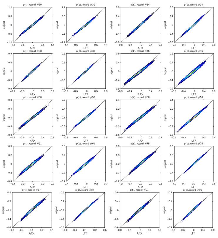
A sample of ARX and LTF simulated wave pressure time series can be observed in Fig. 4. This sample (record #50) was chosen to correspond with the time series presented in Fig. 2. Although, as observed in Table 3, scatter index εs values of ARX simulations are much lower (10~20%), the LTF method performs in most cases better. However, in most cases, the original skewness and kurtosis values are approximated better under ARX than using LTF. In case of pressure simulation, the ARX performance is slightly weaker than the traditional LTF when the model is applied to input data referring to slightly different wave conditions, pressure gauge, water depth and its output is verified against measured data. Basically, simulating pressure records requires filtering out energy in a relevant frequency band; the linear transfer function is a natural solution for this case.
Table 3.
Statistics of free-surface simulation using ARX and LTF compared with original data. Record #38 (in bold) used for estimation
However, if both estimation and validation data are a distinct part of the same time series (which ensures exactly the same meteorological conditions, z and h values), the performance of the ARX simulation is better.
6. Conclusions
System identification procedures were shown to be efficient in the modelling of free-surface records basing on wave pressure record, especially if a low frequency component is included as an additional input time series. This is due to the fact, that the low frequency oscillations are far less attenuated in deep water column than the high frequency components.
Satisfactory performance of SI techniques in low frequency behavior modelling and noise robustness make these methods a good alternative to the corrected LTF method, under the assumption of similar water depth, gauge depth and wave conditions, especially for free-surface simulation. As the Local Polynomial Approximation method is reported to perform similarly to LTF in case of high noiseto-signal ratio, ARX simulation might be locally, when dealing with noisy field data, shown to perform better than LPA. As neither LFA nor LSA have been applied to the field data yet, those methods have not been investigated.


