Measurement of Turbulence Properties at the Time of Flow Reversal Under High Wave Conditions in Hujeong Beach

Yeon S. Chang; Jong Dae Do; Sun-Sin Kim; Kyungmo Ahn; Jae-Youll Jin

doi:10.9765/KSCOE.2017.29.4.206

Journal of Korean Society of Coastal and Ocean Engineers > Volume 29(4); 2017 > Article

후정해변 고파랑 조건하에서 파랑유속 방향전환점에서 발생하는 난류성분의 측정

Article

J Korean Soc Coast Ocean Eng 2017; 29(4): 206-216.

Published online: August 31, 2017

DOI: https://doi.org/10.9765/KSCOE.2017.29.4.206

후정해변 고파랑 조건하에서 파랑유속 방향전환점에서 발생하는 난류성분의 측정

장연식^*, 도종대^**, 김선신^***, 안경모^****, 진재율^*****

Measurement of Turbulence Properties at the Time of Flow Reversal Under High Wave Conditions in Hujeong Beach

Yeon S. Chang^*, Jong Dae Do^**, Sun-Sin Kim^***, Kyungmo Ahn^****, Jae-Youll Jin^*****

^*Coastal Disaster Prevention Research Center, Korea Institute of Ocean Science and Technology

^**Coastal Morphodynamics Section, Korea Institute of Ocean Science and Technology

^***Operational Oceanography Research Center, Korea Institute of Ocean Science and Technology

^****School of Spatial Environment System Engineering, Handong Global University

^*****East Sea Research Institute, Korea Institute of Ocean Science and Technology

Corresponding author: Jae-Youll, Jin, East Sea Research Institute, Korea Institute of Ocean Science and Technology, 787 Haeanro, Ansan 15627, Korea, Tel: +82-54-780-5210, Fax: +82-54- 780-5249, jyjin@kiost.ac.kr

Received August 18, 2017 Revised August 24, 2017 Accepted August 28, 2017

This is an Open Access article distributed under the terms of the Creative Commons Attribution Non-Commercial License (http://creativecommons.org/licenses/by-nc/3.0/) which permits unrestricted noncommercial use, distribution, and reproduction in any medium, provided the original work is properly cited.

요약

교란운동에너지(TKE)와 레이놀즈 응력의 수직성분( −u′w′¯)에 대한 한 주기 파장 안에서의 시간변화를 관측자료를 사용하여 분석하였다. 관측자료는 동해에서 온대성저기압이 발달하였던 2017년 1월 14일부터 18일까지 동해안 후정해변에서 측정한 파랑자료를 사용하였다. 이 기간 동안 관측된 모든 파랑자료들 중에서 비슷한 형태를 갖는 수백 개의 규칙파들을 구분하였으며 이 자료를 토대로 Ensemble Average 기법을 사용하여 이 기간 파랑특성을 대표하는 세 개의 평균파를 계산하였다. 그리고 이 평균파를 기준으로 각 파의 요동을 측정하여 한 주기 동안의 교란운동에너지와 레이놀즈 응력을 계산하였다. 이렇게 계산된 자료들을 분석한 결과 교란운동에너지는 파랑의 평균유속과 비슷한 분포를 나타내었으나(즉 유속이 최대값을 나타낼 때 교란운동에너지도 최대값을 나타내었다), −u′w′¯는 파랑의 수평유속 방향이 전환되는 ‘방향전환점’에서 가파르게 증가하는 경향을 나타내었다. 이러한 −u′w′¯의 독특한 분포는 Nielsen(1992)에 의해 제안된 난류 convection 현상을 뒷받침하는 발견으로 퇴적물과 같은 물질들의 부유현상이 파랑의 ‘방향전환점(한 주기 안에서 파랑의 횡단방향 유속 부호가 바뀌는 시점)’에서 촉진될 수 있음을 보여준다. 이렇게 관측된 난류에너지 분포 특성을 CADMAS-SURF 모델을 사용하여 구현해 보았다. 그 결과 교란운동에너지의 경우 모델결과와 관측치 사이에 유사성이 발견되었으나 레이놀즈 응력( −u′w′¯)의 경우 모델이 ‘방향전환점’에서의 증가현상을 구현해 내지 못하였다. 이는 CADMAS-SURF와 같은 Reynolds-Averaged Navier-Stokes(RANS) 모델들이 가지는 한계점으로 RANS 모델의 경우 레이놀즈 응력과 같은 난류에너지가 평균유속의 분포에 강한 영향을 받기 때문인 것으로 판명되었다.

핵심용어: 레이놀즈 응력, RANS 모델, CADMAS-SURF, 유속방향전환점

Abstract

The temporal distribution of the turbulence kinetic energy (TKE) and the vertical component of Reynolds stresses ( −u′w′¯) was measured during one wave period under high wave energy conditions. The wave data were obtained at Hujeong Beach in the east coast of Korea at January 14~18 of 2017 when an extratropical cyclone was developed in the East Sea. Among the whole thousands of waves measured during the period, hundreds of regular waves that had with similar pattern were selected for the analysis in order to give three representing mean wave patterns using the ensemble average technique. The turbulence properties were then estimated based on the selected wave data. It is interesting to find out that −u′w′¯ has one clear peak near the time of flow reversal while TKE has two peaks at the corresponding times of maximum cross-shore velocity magnitudes. The distinguished pattern of Reynolds stress indicates that vertical fluxes of such properties as suspended sediments may be enhanced at the time when the horizontal flow direction is reversed to disturb the flows, supporting the turbulence convection process proposed by Nielsen (1992). The characteristic patterns of turbulence properties are examined using the CADMAS-SURF Reynolds-Averaged Navier-Stokes (RANS) model. Although the model can reasonably simulate the distribution of TKE pattern, it fails to produce the −u′w′¯ peak at the time of flow reversal, which indicates that the application of RANS model is limited in the prediction of some turbulence properties such as Reynolds stresses.

Keywords: Reynolds stress, RANS model, CADMAS-SURF, flow reversal

1. Introduction

The Reynolds stresses (레이놀즈 응력) is the stress tensor that arises when the Navier-Stokes equations are Reynolds averaged by decomposing the velocity field into mean and fluctuation parts as

(1)

ui=u¯ι+ui'

where u_i is the fluid velocity in i direction and ui and ui'are the averaged velocity and velocity fluctuation respectively. When Eqn. (1) is inserted into the Navier-Stokes equation and then averaged, the Reynolds-Averaged Navier Stokes (RANS) equation can be written as

(2)

∂u¯ι∂t+uJ∂u¯ι∂xj=−1ρ∂p¯∂xi+∂∂xj(ν∂u¯ι∂xj−uι'uJ'¯)

where r is the fluid density (밀도), p is pressure (압력) and ν is the kinematic viscosity (동점성계수).

In Eqn. (2), the product of velocity fluctuation is the Reynolds stresses as

(3)

Rij=−uι'uJ.'¯

where the overbar denotes the average of the products of velocity fluctuation in time. As shown in Eqn. (2), the Reynolds stresses are the additional forces to the mean flow generated by the turbulent fluctuations. These stresses play important role as they can produce momentum fluxes in the direction perpendicular to the mean flows. In the boundary layer, for example, the vertical component of Reynolds stresses, −u′w′¯, produces vertical flux caused by the fluctuation of horizontal momentum.

Such vertical fluxes are specifically important in the study of sediment transport in coastal regions. In the unsteady boundary layers under oscillating wave conditions, the sediments are suspended from the seabed by the turbulent eddies and the upward sediment fluxes can be described by the Reynolds stress, −u′w′¯ (Nielsen, 1992). The precise quantification of this Reynolds stress is, however, difficult as it is a correlation of fluctuated velocity components from the mean value, (u-u)(w-w), which blocks the closure of Eqn. (2). The most popular postulation to model the Reynolds stresses to close the system is the Boussinesq eddy viscosity approximation (Boussinesq, 1877; Schmitt, 2007) by which the Reynolds stress tensor is assumed to be proportional to the mean strain rate tensor (평균 변형텐서) as

(4)

Rij=2νtSij−2/3kδij

where ν_t is the kinetic eddy viscosity,k is the turbulent kinetic energy (TKE, 교란운동에너지) ( k=12ul'ul'), δ_ij is the Kronecker delta, and S_ij is the mean strain rate tensor ( Sij=∂ul∂xj+∂uJ∂xi) that measures the rate of mean flow deformation. Therefore, Eqn. (4) implies that Reynolds stresses can be expressed in terms of the spatial variation of the mean flow velocities. The advantage of the Boussinesq approximation (부씨네스크 근사) is that Eqn. (2) is closed using the concept of turbulent eddy viscosity (난류 와동 점성), ν_t, which generates the RANS turbulence modeling system (Wilcox, 1998). As one example, the k − ε RANS model closes the system by solving two additional equations of TKE (k) and dissipation (ε) using νt~k²/ε (Lauder and Spalding, 1974).

The RANS models have successfully applied to simulate various turbulent flows (Rodi, 2017). However, the performance of several RANS models that applied to pulsating turbulent boundary layers showed discrepancies in turbulence quantities such as Reynolds stresses during some part of oscillating cycles while it gave satisfactory description of mean streamwise velocities (Scotti and Piomelli, 2001). In addition, Chang and Scotti (2004) observed that a RANS model underestimated the Reynolds stress, u'w', over a rippled bed in oscillating boundary layer flows while this quantity was essential in modeling sediment suspension process. The discrepancy in the turbulent eddy viscosity approximation was not only found in the magnitude of turbulence energy but also in the timing of maximum energy rates (Chang and Scotti, 2006). Since the Reynolds stresses are proportional to the mean velocity gradient in the Boussinesq approximation, the temporal variation of −u′w′¯ follows the pattern of mean velocities as the turbulence energy becomes minimal at the time of flow reversal (방향전환점) when the mean velocity diminishes in oscillating unsteady boundary layer flows (Chang and Park, 2016). This may cause discrepancies in the time distribution of sediment suspension pattern because sediments are also suspended during the time of flow reversals (O’Donoghue and Wright, 2004; Chang and Scotti, 2006). The sediment suspension peaks at flow reversals were previously investigated using the ‘sediment convection (대류)’ concept (Nielsen, 1992). While the exiting sediment distribution models used the ‘sediment diffusion (확산)’ to describe the sediment suspension process by which the maximum suspension rates occurred at the time of maximum mean flow rates, the convective sediments were picked-up from the bed according to turbulent energy distribution (Amoudry et al., 2016; Chang et al., 2017). In order to include the convection process in modeling sediment transport, therefore, it is important to closely examine the structure and temporal distribution of the Reynolds stresses by testing the Boussinesq approximation specifically under pulsating unsteady wave conditions, which has been rarely studied due to the difficulties of in-situ measurement of turbulence quantities under wave conditions.

In the present study, we propose to examine the temporal distribution of u'w' using the high frequency acoustic instrumentation under high wave energy conditions in a nearshore region of the east coast of Korea. The purpose of this study is then to investigate the structure of Reynolds stresses that significantly contribute to the upward sediment flux during the wave period. This study is important because the timing of the peak flow turbulence energy can greatly affect the cross-shore (횡단방향) sediment transport pattern as it determines the peak time of sediment suspension during one wave period. In addition, we propose to diagnose a RANS model for the performance of the generation of turbulence energy in order to support the previous study results.

2. Field Experiment and Data Analysis

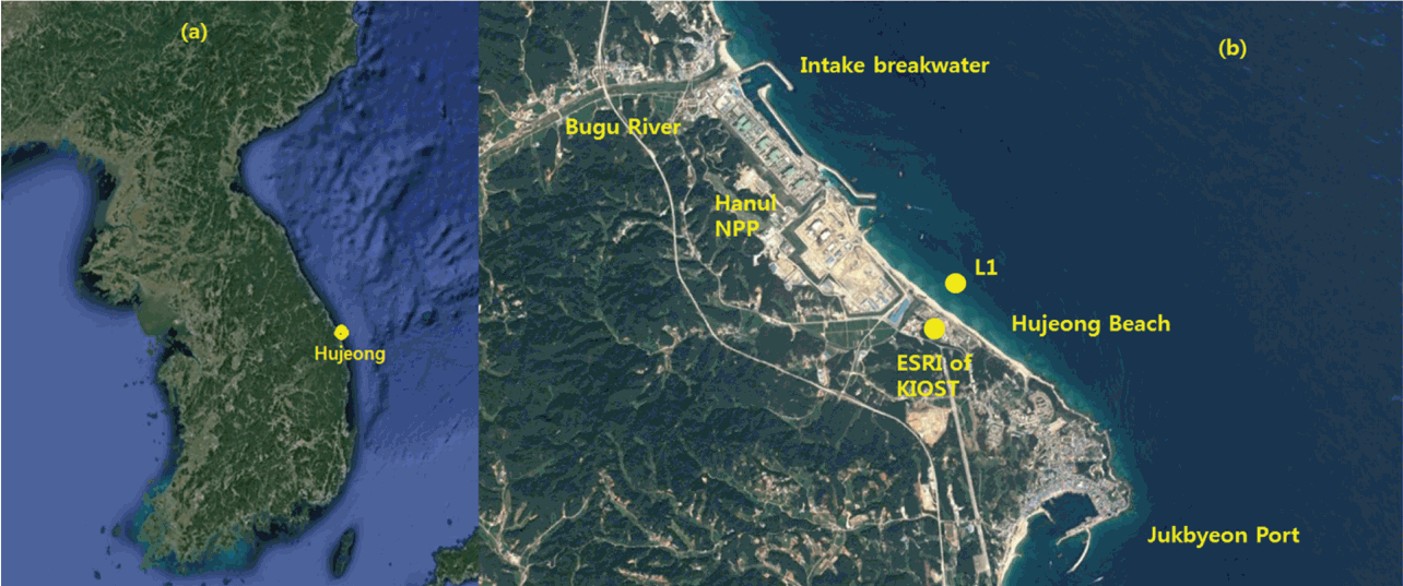
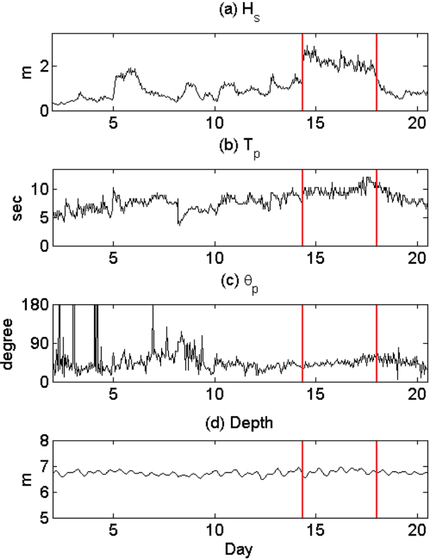
Hujeong Beach (후정 해변) is located in the east coast of Korea between Jukbyeon Port (죽변항) and Bugu River (부구천) (Fig. 1). It is about 3 km long sand beach facing the northeast. In the northern end of the beach, the breakwater to protect the intake of Hanul Nuclear Power Plant (NPP, 한울원자력발전소) is located blocking the sediment discharge from the Bugu River. While it has microtidal environment with tidal range of a few decimeters only, the east coast of Korea suffers from storm waves during winter due to the movement of extratropical cyclone (온대 저기압) from China to the East Sea as the swell-like high waves usually attack the coasts during the period from October to February (Jeong et al., 2007, 2016). For this reason, the East Sea Research Institute (ESRI, 동해연구소) of Korea Institute of Ocean Science and Technology (KIOST, 한국해양과학기술원) that is located in the Hujeong Beach measured waves, currents and turbulence during January, 2017 at the location, ‘L1’ where water depth varies 6.5~7.0 m (Fig. 2(c)). The flow velocities are measured using a Vector, 3-dimensional acoustic velocimeter that is designed for turbulence and wave measurements. The velocimeter was moored at about 0.25 m above the bed while the pressure sensor was moored at about 0.65 m above the bed. The sampling frequency of the flow velocities is 2 Hz while the sampling frequency of pressure sensor is 1 Hz. During the period, the data were sampled for 20 minutes at every hour, which gives 24 data bursts per day as each burst contains the 20-minute data.

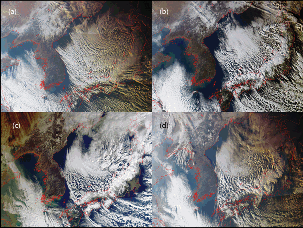
Fig. 2(a)~2(c) show the significant wave heights (H_s), peak wave period (T_p) and the peak wave directions (θ_p) averaged over each data burst from January 2 to 20. H_s are lower than 2 m at most of the dates. However, it sharply increases higher than 2 m at January 14. The high wave condition continues until January 18 during which H_s varies between 2.0~2.7 m. After January 18, H_s sharply decreases below than 2 m. In case of T_p, it increases from about 5 sec at January 2 and, during the period from January 14 to 18, it varies between 8 and 10 sec. In this period, θ_p slightly varies around 45o indicating that the waves mainly approached the shore from northeast (90o is the shore normal direction). The high waves with the uniform northeast approaching direction at January 14~18 are likely the storm waves (폭풍파) caused by the extratropical cyclone developed in the northeast of the East Sea as shown in the satellite images of Geostationary Ocean Color Imager (GOCI) in Fig. 3. In the present study, we focus to examine the energy distribution of the waves measured during this storm period. The main reason for the analysis of the data selected at this time is because the characteristics of turbulence energy pattern are more clearly observed under high wave conditions in which the flows are strongly disturbed by the unsteady pulsating wave conditions. In addition, under swell-like high wave conditions, individual waves can be more easily distinguished during each wave period while, under lower wave energy conditions, individual waves are not easily separated because the waves are irregular due to the interference between the waves. For this reason, we selected the data from January 14 to 18 for the investigation of this study as this period is marked with the red vertical lines in Fig. 2.

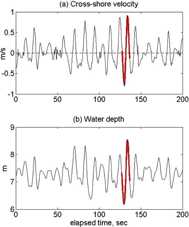
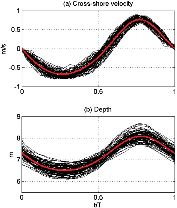
The analysis of the wave data is performed using the ensemble average technique (Chang and Hanes, 2004). In the first step of this process, the individual waves that have clear wave pattern are selected. For example, Fig. 4 shows time series of cross-shore velocity and pressure data for 100 seconds during which 16 wave crests are observed. During each wave period, however, most of the waves do not show clear wave pattern that has one crest and one trough with similar magnitude. Instead, many waves show multiple peaks during its period or the magnitude of crest and trough shows severe discrepancies, which may contaminate the energy distribution during one the period of those irregular and asymmetric waves. In spite of the irregularity (불규칙성) of the measured data, we could still find one regular wave (규칙파) during this time that has a clear crest and a trough with symmetric magnitude as marked in red color in Fig. 4. During the storm period between January 14 and 18, we could find total 239 waves that has clear regular wave pattern. These regular waves have similar wave pattern as they have similar wave periods with the mean period (T_m) to be 10.2 sec and the standard deviation to be 0.9 sec.

In order to capture these individual waves from the time series data, we used the cross-shore velocity time series in Fig. 4(a). First, we found the zero-crossing points of the selected regular waves when the cross-shore velocity changed its sign from positive (onshore) to negative (offshore), which gave one wave period when the two adjacent onshore-tooffshore zero-crossing points were measured. Once the zero-crossing points were obtained, we then interpolated all the selected regular waves that have different wave periods by normalizing the time by the period of each individual regular wave, t/T. Since these selected waves have similar periods around 10 sec, the normalization would not produce serious errors in the ensemble average caused by the difference of the wave periods. Through these processes, we could obtain 239 individual waves (개별파) that have same normalized period as t/T varies 0 to 1. The whole individual regular waves were then divided into 3 groups according to its maximum velocity at wave crest. In Group 1, the 89 waves whose maximum onshore velocities are between 0.4~0.6 m/s were chosen. In Group 2, the 88 waves whose maximum onshore velocities are between 0.6~0.8 were chosen, and the rest 62 waves with onshore maximum velocities between 0.8~1.0 belonged to Group 3. In Fig. 5, the cross-shore velocities and pressure of the individual waves of Group 2 are plotted with solid black solid lines. As shown in the figure, the waves in the same group show similar wave pattern, which enables the measurement of turbulence parameters for each group. The red lines in Fig. 5 show the mean wave patterns of cross-shore velocity and pressure representing the group.

3. Model Description and Numerical Experiment

The RANS model used in this study is the two-dimensional CADMAS-SURF developed by the Port and Harbor Research Institute (PHRI), Japan (2001). The model can simulate the wave and structure interaction in a wave channel using k − ε turbulence closure model. The model is characterized by the Volume of Fluid (VOF) method that tracks and locates the free surface by solving additional advection equation for a fluid volume function (Hirt and Nichols, 1981; Hieu and Tanimoto, 2006). The CADMASSURF model has been successfully on wave run-up (처오름) problems on porous seabeds (투과성 해저면) (Nam et al., 2002; Yoon et al., 2005).

The continuity as well as momentum equations of the model are the Navier-Stokes equation that is expanded for porous body as

(5)

∂γxu∂x+∂γzw∂z=Sp

(6)

λν∂u∂t+∂λxuu∂x+∂λzwu∂z=−γvρ∂p∂x+∂∂x{γxνe(2∂u∂x)}+∂∂z{γzνe(∂u∂z+∂w∂x)}−Dxu+Su−Rx

(7)

λν∂w∂t+∂λxuw∂x+∂λzww∂z=−γvρ∂p∂z+∂∂x{γxνe(∂w∂x+∂u∂z)}+∂∂z{γzνe(2∂w∂x)}−Dzw+Sw−Rz−γνg

where u and w are the horizontal and vertical flow velocities, ρ is fluid density, p is pressure, g is gravitational force, ν_e is eddy viscosity (와동 점성계수), D_x and D_z are the energy attenuation coefficients (에너지 경감 계수), γ_ν is porosity (다공성), γ_x and γ_z are the area transmittance (투과율) in the x and z direction respectively. λ_ν, λ_x and λ_z are functions of γ_ν, γ_x and γ_z respectively as they are expressed as

(8)

λν=γν+(1−γν)CMλx=γx+(1−γx)CMλz=γz+(1−γz)CM

where C_M is the inertia coefficient (관성계수). R_x and R_z are the resistance force (저항력) applying quadratic law as

(9)

Rx=12CDΔx(1−γx)uu2+w2Rz=12CDΔz(1−γz)wu2+w2

where Δx and Δ_z are the grid size in the x and z direction respectively and C_D is the drag coefficient (항력계수). S_p, S_u and S_z are the source terms to generate the wave conditions.

The VOF method is applied to simulate free surface generation by solving the advection equation of a fluid volume function, F, that varies between 0 to 1. The 1 value of F at a grid cell indicates that the cell is filled with fluid while 0 value indicates that fluid is empty in the cell. When F is greater than 0 but smaller than 1, the grid cell is partly occupied by fluid indicating that the cell is located at the boundary between the fluid and air. The advection equation of F is given as

(10)

γν∂F∂t+∂γxuF∂x+∂γzwF∂z=SF

where S_F is source term to generate wave conditions. In order to close the equations from (5)~(7), k − ε model is employed to calculate the eddy viscosity, ν_e, as

(11)

γν∂k∂t+∂γxuk∂x+∂γzwk∂z=∂∂x{γxνk(∂k∂x)}+∂∂z{γzνk(∂k∂z)}+γvGs−γνε

(12)

γν∂ε∂t+∂γxuε∂x+∂γzwε∂z=∂∂x{γxνε(∂ε∂x)}+∂∂z{γzνε(∂ε∂z)}+γvC2εkGs−γνC2ε2k

(13)

Gs=νt{2(∂u∂x)2+2(∂w∂z)2+(∂w∂x+∂u∂z)2}

where C₁ and C₂ are empirically determined coefficients (경험계수), and the relations between ν_k, ν_ε, ν_t and ν_e are given as

(14)

νt=Cμk2ε,νk=ν+νtσk,νε=ν+νtσε and νe=ν+νt

where C_μ, σ_k, σ_ε are empirically determined coefficients.

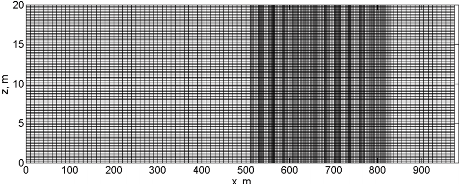
The above RANS equations are solved to simulate the experimental conditions described in section 2. The computational domain is a 2-dimensional rectangular channel with length of 984 m and height of 20 m (Fig. 6). The horizontal grid size varies from 1.0 m to 0.1 m because fine resolution is required near the surf zone. In the vertical direction, the grid size is set to be constant value with 0.2 m throughout the water column, which is fine enough to resolve the turbulence energy near the bed when imposing the no-slip bottom boundary condition. An ideal case of regular wave condition is generated by imposing the wave height to be 2.5 m at the source with 10 sec wave period at 7.3 m water depth in order to generate similar condition to the observed waves shown in Fig. 2. The waves are generated using Stokes wave approximate solutions at the source and the source is located at x = 328 m as it is determined considering the wave length. At the open boundary, the Sommerfeld radiation condition and a damping zone are applied to reduce the reflection effect. At the bottom boundary, the porous seabed condition is not applied as it may affect the near bed flows when applying the inertia and drag coefficients as they are defined in Eqn. (8) and (9).

4. Results

4.1 Reynolds stress distribution

The 3 groups of wave data sets obtained from the ensemble average method described in Section 2 are used to calculate the turbulence properties such as turbulence kinetic energy ((TKE=((u'2)+(ν'2)+(w'2))/2)) and the vertical component of Reynolds stress ( −u′w′¯) of which the importance is explained in Section 1. Since these turbulence parameters contain fluctuation components, it should be careful in measuring such quantities because they are the deviations from the mean values. Therefore, the accuracy of the estimation of fluctuated components depends on the measurement of the mean values as u'=u-u. In this experiment, we elaborated to calculate the mean velocities by strictly selecting the regular waves for each group. In addition to the maximum onshore velocities, we also consider the maximum offshore velocities for the maximum magnitude of velocity difference between waves (Δu_max) not to be larger than 0.2 m/s. Moreover, we also consider the wave asymmetry (비대칭도) and skewness (왜곡도) as [(u_max)_onshore − (u_max)_offshore]/(u_max)_onshore of each selected regular wave are monitored to be less than 10% and the times of offshore-to-onshore zero-crossing points of the waves are also to be concentrated within 10% range from the mean values.

From the data sets of the waves selected based on the above criteria, we calculated the TKE and −u′w′¯ for the 3 groups during the normalized wave period as shown in Fig. 7. As it was designed, the maximum magnitudes of the averaged cross-shore velocities gradually increase from Group 1 to Group 3 by 0.2 m/s. The magnitude difference, (u_max)_onshore − (u_max)_offshore, is also about 0.1 m/s for all three groups. In addition, the times of offshore-to-onshore zerocrossing points occur at t/T~0.55 for all three groups. Another similarity is also found in the oscillating periods as the averaged times for the cross-shore velocity to cycle between the two adjacent zero-crossing points are 10.1, 10.1 and 10.3 sec for Group 1, 2 and 3 respectively. These similarities between the cross-shore velocity patterns between the three groups of the selected waves indicate that the only significant difference is the maximum velocity magnitude, and the similar wave pattern enhances the accuracy of turbulence measurement at this time.

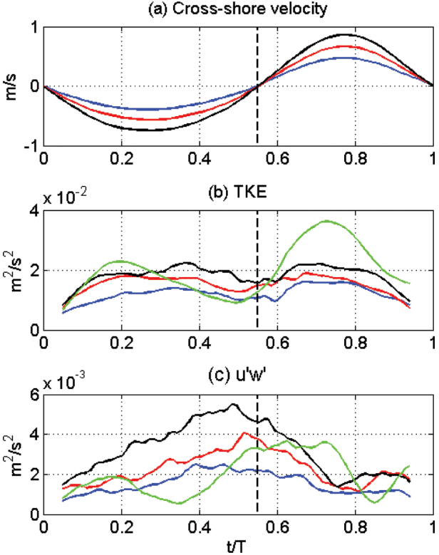
In Fig. 7(b), the TKE distribution is compared between the three groups. The maximum TKE magnitudes also increase as the maximum velocity magnitude increases. In addition, the TKE of all three groups show two peaks during the normalized period as they roughly correspond to the time of maximum offshore and onshore cross-shore velocities, showing that the turbulence energy varies correspondingly to the mean flow energy during the wave period. This pattern of TKE with two peaks at maximum crossshore flow rates is similar to the model results over flat bottom by Chang and Hanes (2003), which indicates that the morphological effect of seabed does not significantly affect the turbulence measurement of this study.

One interesting founding that is distinguished from the velocity pattern is observed in the vertical component of Reynolds stress distribution (Fig. 7(c)). Unlike the TKE distribution, −u′w′¯ distribution has one peak near the time of offshore-to-onshore zero-crossing point during the normalized wave period the turbulence flux for all three wave groups though the magnitude of their peaks increase with the maximum flow rates. The results of TKE and −u′w′¯ show that the vertical turbulence flux becomes strong when the horizontal flow is reversed (when the streamwise flow changes its direction from offshore to onshore) while the turbulence energy is strong at the time of maximum flow rates (when the cross-shore velocity magnitude has two peaks). This also indicates that the suspended sediments can be strongly moved in the vertical direction at this time of flow reversal. This finding from turbulence measurements is important because it supports the convection process studied in the previous experiments (Nielsen, 1992; O’Donoghue and Wright, 2004; Chang and Scotti, 2006). Unlike the diffusion process that suspends the sediments from bed when the TKE becomes maximum at the times of maximum flow rates, the convection process entrains the sediments at the time of flow reversal when the flows are disturbed when the streamwise flow changes its direction and the organized coherent flow turbulence structures are broken to scatter the structures not only to the horizontal direction but also to the vertical direction as well (Chang and Scotti, 2006; Chang et al., 2016).

In measuring the turbulence quantities, one of the weaknesses of the ensemble average technique used in this study is the possible underestimation/overestimation of the turbulence magnitude by the pseudo-turbulence. As shown in Fig. 5, the turbulence quantities are calculated by measuring the difference between the selected wave velocities (black lines) and their phase-averaged value (red line). This may still involve the mean components in the turbulence measurements as they are caused by the shift in the velocity magnitudes, which needs to be distinguished from the pure turbulent components. Another common approach to measure the turbulence quantities is the high-pass filtering that removes the components that are lower than the cut-off frequency. By doing this, the mean velocity components are filtered and the high frequent turbulent motions are to be measured. The green lines in Fig. 7(b) and (c) are the TKE and u'w' measured by the high-pass filtering method averaged over the 239 selected regular waves by setting the cutoff frequency at 1 Hz. As shown in the figure, the patterns of the turbulence quantities show difference from those measured by the ensemble average technique. For example, the magnitudes of the high-pass filtered TKE are bigger and its peak values are also clearly different at the onshore and off-shore phases. In addition, the timing of the u'w' peaks shows phase difference as the peak of the highpass filtered occurs later compared to the peaks of the ensemble averaged values. This difference between the two measures is not clear, but it is likely that the high-pass filtered turbulence quantities also involve mean components. The cut-off frequency has to be set at 1 Hz due to the velocity measurements with 2 Hz, which may be too low to clearly separate the turbulence components only. It should be noted, however, that both of the ensemble averaged and high-pass filtered u'w' increase at the time of flow reversal at t/T = 0.55 while TKE of both measures do not show peaks at this time. This supports the results that the increment of the vertical component of the Reynolds stresses at the time of the flow reversal due to the disturbance of flows when the streamwise flow changes its direction.

4.2 Model comparison

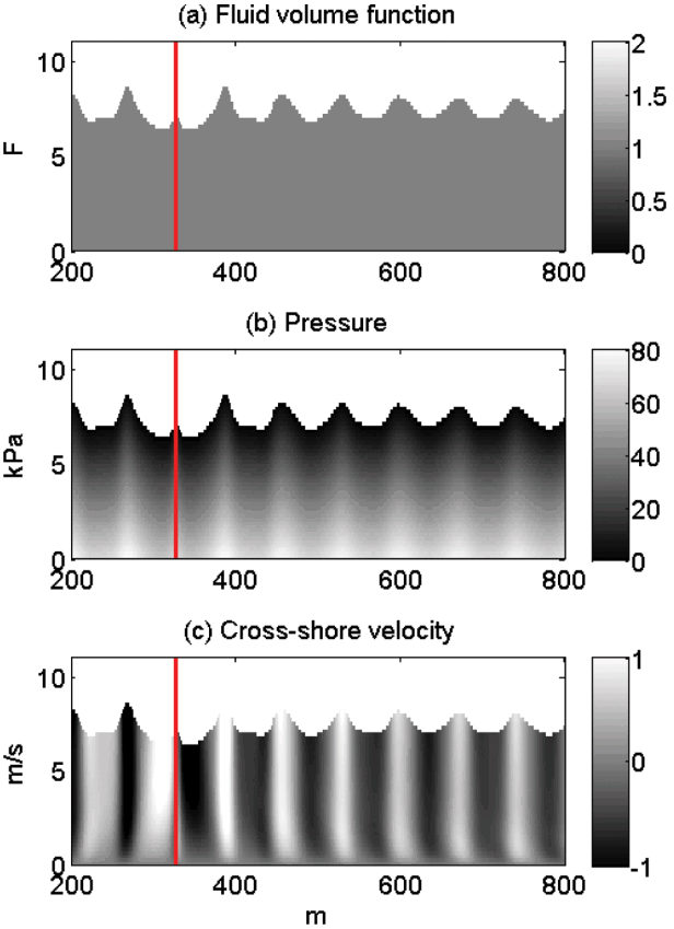
Fig. 8 shows a schematic of the wave propagation calculated by the CADMAS-SURF by contouring the fluid volume function (F), water pressure (P) and the cross-shore velocity (u) as they are calculated from Eqn. (6) and (10). The red vertical line in the figure denotes the location of the source where the wave generation condition is imposed. The figures show that the model nicely simulates the propagated wave trains on the flat bed. Near the bottom boundary layer below 1 m, the cross-shore velocities show time lags from the velocities in the upper layers due to the bottom drag.

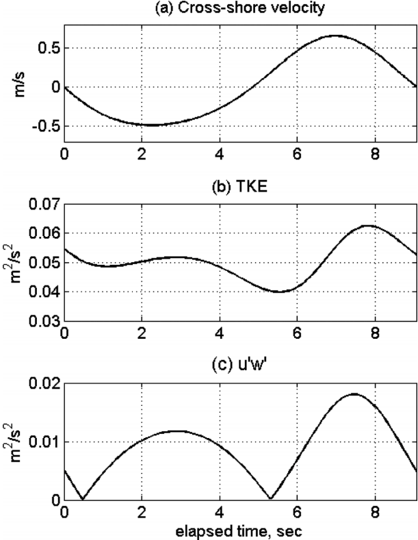
In order for a comparison with the observed data, we sampled the CADMAS-SURF data at the location of x = 500 m and z = 0.4 m above the bed as the grid cell of this location is closest to the location of the observation as described in section 2. Fig. 9 shows the cross-shore velocity, TKE and the magnitude of vertical component of Reynolds stress distribution (u'w') distribution over the normalized wave period as they are calculated from CADMAS-SURF. The Reynolds stress is estimated using the formula described in Eqn. (4). It should be noted that the shape of the crossshore velocity pattern is similar to that of the measured velocities in Fig. 7(a) as both of the maximum on-shore and offshore velocity magnitudes are similar to the measured magnitudes of the Group 2 waves, showing that the wave asymmetry is nicely resolved by the model. In addition, the wave skewness is resolved by the model as the zero-crossing point of the modeled velocity also occurs at t/T~0.55 corresponding to the measurements. In spite of the success in the generation of the averaged cross-shore velocity pattern, the turbulence parameters, TKE and u'w', are not well simulated by the model. First of all, the magnitudes of these quantities are severely overestimated. This overestimation in the magnitudes by the model is not clearly understood. However, it is likely that the 2-dimensinality of the model may cause problems in measuring the 3-dimensional turbulence quantities. The turbulent flow motions in the bottom boundary layers are fully 3-dimensional as the velocity fluctuations not only develop in the streamwise direction but also in the directions perpendicular to it. Therefore, the 2-dimensional (streamwise-vertical) models may not correctly capture the turbulence quantities. The error in these 2-dimensional models may be reduced by tuning the model coefficients as such of them are listed in Eqn. (14) for the present model configuration. These coefficients were, however, empirically determined from limited applications and thus not tuned for this specific experiment. The tuning of these coefficients is out of the scope of the present study, and may remain for future studies. Instead, we focus on the discrepancy in the timing when the turbulence parameters have peaks. As already mentioned, the TKE distribution of the measured data has two peaks at corresponding times of the maximum flow rates (Fig. 7(b)) u'w' while the observed distribution has one peak at the time of flow reversal (Fig. 7(c)). The model results show that both of the TKE and u'w' have two peaks near the time of maximum flow rates (Fig. 9(b) and (c)). The two peaks in TKE of the model results are similar to that of the observed data. However, the magnitude of the peak at the on-shore wave phase is greater than that of the peak at the offshore phase. The difference in the magnitude is likely caused by the asymmetry in the velocity magnitude, which was not found in the observed data. The discrepancy in the distribution is more significant as two clear peaks that correspond to the times of maximum flow rates are found in the modeled Reynolds stress. The magnitudes of the two peaks of u'w' are also different as that of the on-shore wave phase is greater than that of the offshore phase. The discrepancy in the timing of u'w' peaks during wave period may cause significant difference in the vertical momentum flux, which may resulted in unexpected error in the prediction of net transport of materials such as suspended sediments.

5. Conclusion

In this study, we compared the temporal distributions of turbulence quantities of TKE and u'w'between the ensemble-averaged observation data and model results. It shows that the waves are slightly asymmetric and skewed under high wave conditions during the winter time storm period at Hujeong Beach, which was successfully generated by the CADMAS-SURF RANS model. However, it is interesting to find out that the observed Reynolds stress had one clear peak at the time when the streamwise flow changed its horizontal direction. This peak of turbulence quantities at the time of flow reversal was not simulated by the model.

The result shows an important indication in the study of transport of materials such as sediments in the nearshore region. Nielsen (1992) proposed a concept of turbulence convection process by which sediments are picked from the bed by flow turbulence in more organized way than the diffusion process by which the sediments are dispersed into the water column by the near-bed sediment concentration gradient. While the diffusion process is strong during the time of maximum flow rates, the convection process may be strong when the flow turbulent structures are active at such times of flow reversal. The observation of the peak u'w' of at the time of flow reversal in the present study is important as it can support the concept of convection process which has not been correctly modeled in the sediment suspension models yet.

Another important result of this study is that a failure of a RANS model to produce the turbulence convection at the time of flow reversal as u'w' of the model shows two peaks at the time of maximum flow, not at the time of flow reversal. This is likely due to the formulation of the Reynolds stresses in terms of mean flow gradients. As described in Eqn. (4), the Reynolds stresses are expressed in terms of the gradient of mean flow velocities (S_ij). Therefore, the development of these turbulence quantities strongly depends on the mean flow pattern, which may not correctly describe the turbulence pattern at the time of flow reversal when the mean velocity diminishes. To overcome this problem, additional contributions may be necessary in formulating the turbulence quantities under high wave energy conditions, which is suggested for future studies.

감사의 글

This study was funded by Korea Institute of Ocean Science and Technology (KIOST, PE99523).

Fig. 1.

(a) the location of Hujeong Beach in the east coast of Korea. (b) The map of the Hujeong Beach and the location of ‘L1’ where the instruments were moored during the experiment period from January 2∼20, 2017. The maps of the figure are captured from Google Earth.

Fig. 2.

Significant wave heights (H_s), peak wave period (T_p), peak wave direction (θ_p), and the water depth estimated from the pressure sensor averaged over each 10-minute data burst in January 2∼20.

Fig. 3.

Satellite image of Geostationary Ocean Color Imager (GOCI) at (a) 07:00, January 14, 2017; (b) 06:00, January 15, 2017; (c) 00:00, January 16, 2017; (d) 07:00, January 16, 2017. It shows that an extratropical cyclone is developed in the northeast of the East Sea.

Fig. 4.

An example of time series data of cross-shore velocities and pressure for 100 seconds. The red color marks the individual regular wave that is selected for the ensemble average.

Fig. 5.

Black lines – the cross-shore velocities and pressure of individual waves in Group 2 during the normalized wave period, t/T. Red lines – the mean cross-shore velocity and pressure that represent the pattern of Group 2 waves.

Fig. 6.

Computational domain of the CADMAS-SURF modeling system.

Fig. 7.

Measured cross-shore velocity, TKE, and Reynolds stresses ( −u′w′¯) for each group during normalized wave period. Blue – Group 1 (ensemble averaged), red – Group 2 (ensemble averaged), black – Group 3 (ensemble averaged), green – high-pass filtered.

Fig. 8.

Schematic of wave propagation resulted from CADDMAS-SURF. (a) contour of the fluid volume function, F, (b) water pressure, (c) cross-shore velocity. The red line denotes the location of the source where the waves are generated.

Fig. 9.

Modeled cross-shore velocity, TKE, and Reynolds stresses ( −u′w′¯) by CADMAS-SURF during normalized wave period.

References

Amoudry, LO, Souza, AJ, Thorne, PD, Liu, P. (2013). Toward representing wave-induced sediment suspension over sand ripples in RANS models, J. Geophys. Res., 118(1):658-673.

Boussinesq, J. (1877). Essai sur la théorie des eaux courantes, Mémoires présentés par divers savants à l’Académie des Sciences, 23(1):1-680.

Chang, YS, Hanes, DM. (2004). Suspended sediment and hydrodynamics above mildly sloped large wave ripples, J. Geophys. Res, 109(C7.

Chang, YS, Hwang, JH, Park, Y-G. (2017). Sensitivity of suspension pattern of numerically simulated sediments to oscillating periods of channel flows over a rippled bed, KSCE J. Civil Eng., 21(5):1503-1515.

Chang, YS, Park, Y-G. (2016). Suspension of sediment particles over a ripple due to turbulent convection under unsteady flow conditions, Ocean Sci. J., 51(1):127-135.

Chang, YS, Scotti, A. (2004). Modeling unsteady turbulent flows over ripples: Raynolds-averaged navier-stokes equations (rans) versus large-eddy simulation (les), J. Geophys. Res, 109(C9.

Chang, YS, Scotti, A. (2006). Turbulent convection of suspended sediments due to flow reversal, J. Geophys. Res, 111(C07001.

Hieu, PD, Tanimoto, K. (2006). Verification of a VOF-based two-phase flow model for wave breaking and wave-structure interactions, Ocean Engineering, 33, 1565-1588.

Hirt, CW, Nichols, BD. (1981). Volume of fluid (VOF) method for the dynamics of free boundaries, J. Computational Physics, 39, 201-225.

Jeong, WM, Oh, S-H, Lee, DY. (2007). Abnormally high waves on the east coast, J. Korean Soc. Coastal and Ocean Engineers, 19(4):295-302 (in Korean).

Jeong, WM, Ryu, K-H, Oh, S-H, Baek, WD. (2016). Trend of storm wave appearance on the east coast analyzed by using long-term wave observation data, J. Korean Soc. Coastal and Ocean Engineers, 28(2):109-115 (in Korean).

Launder, BE, Spalding, DB. (1974). The numerical computation of turbulent flows, Computer Methods in Applied Mechanics and Engineering, 3(2):269-289.

Nam, I-S, Yoon, H-S, Kim, J-W, Ryu, C-R. (2005). Numerical modeling of wave run-up and internal set-up on and in permeable coastal structure, Journal of Advanced Research in Ocean Engineering, 16(5):34-40.

Nielsen, P. (1992). Coastal bottom boundary layers and sediment transport. 4: World Scientific, River Egde, NJ.

PHRI, Coastal Development Institute of Technology. (2001). Research and development of numerical wave channel (CADMAS-SURF), CDIT Library, 12.

Rodi, W. (2017). Turbulence modeling and simulation in hydraulics: a historical review, J. Hydraulic Eng., 143(5):1-20.

Schmitt, FG. (2007). About Boussinesq’s turbulent viscosity hypothesis: historical remarks and a direct evaluation of its validity, Comptes Rendus Mécanique, 335(9–10):617-627.

Scotti, A, Piomelli, U. (2001). Numerical simulation of pulsating turbulent channel, Phys. Fluids, 13(5):1367-1384.

Wilcox, CD. (1998). Turbulence Modeling for CFD. 2nd Ed. DCW Industries, La Cañada: ISBN 0963605100.

Yoon, H-S, Cha, J-H, Kang, Y-K. (2005). An application of CADMAS-SURF to the wave run-up in permeable coastal structures, Journal of Advanced Research in Ocean Engineering, 19(4):49-55.