


1. Introduction
In the East Sea (ES) during winter, mean surface winds over the sea are northwesterly and generally strong due to two synoptic-scale features, the Siberian High and the Aleutian Low, under the context of the cold and dry East Asian winter monsoon. Storm waves due to winter storms (e.g. extratropical cyclones) in the winter ES are frequently reported causing extensive coastal damages along the coasts of Korea and Japan.
In February 2008, high storm waves due to a developed low propagating from the west off Hokkaido to the south and southwest in the ES caused extensive damages along the coasts of Korea and Japan. The observed maximum wave heights and periods are appeared in Table 1. The high storm waves propagated into the Toyama Bay, Japan, caused one of the most severe coastal damages ever induced by such conditions. In particular, the Fushiki Port in the Toyama Bay experienced large damages in its North-Breakwater due to the high storm waves. The storm waves were refracted by the local bathymetry, and then wave energies were concentrated on certain parts of the North-Breakwater, resulting in the damaged blocks. Such storm waves in the Toyama Bay are called as Yorimawari Waves by the local people and investigated by Lee et al. (2010) on their generation mechanisms by literature reviews and numerical experiments.
Table 1.
Observed maximum wave heights, periods and time in February 2008 due to a developed low. Data are from NOWPHAS, Japan (JP), and KHOA, Korea (KR)
Recently in 3~5 April 2012, an extratropical cyclone being developed to 964 hPa in its intensity at 20:00 UTC 3 April during its passage over the ES brought record-breaking significant wave heights along the west coast of Tohoku, Japan. The observed significant wave heights by GPS wave buoys at Akita and Yamagata were 11.21 m and 12.39 m and the significant wave periods were 13.6 sec and 14.3 sec, respectively, which both were the maximum wave heights and periods ever recorded in the ES due to a winter storm. Huge coastal damages were reported along the west coast of Tohoku, Japan, by the high storm waves. Lee (2013a) reported the physical process of rapid intensification of the low pressure such that the moving low was intensified by the enhanced local convection due to the large latent heat and vapor supply from the extended Tsushima Warm Currents in the ES.
In addition, Lee et al. (2010) and Lee and Yamashita (2011) investigated past events of the winter storms and storm waves in the ES and demonstrated three representative meteorological patterns of developing low pressures in terms of their moving paths (Fig. 1).
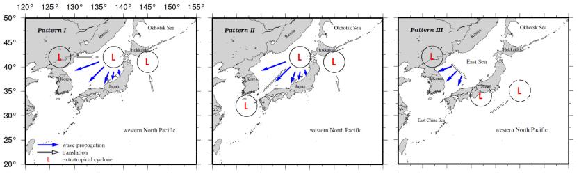
(Pattern I) A low pressure in the continent in the west of Korean Peninsula moves toward east, while being developed over the ES. Another low pressure is being developed and located in the east of Hokkaido, Japan, over the Pacific Ocean. Due to the interaction between the two lows, the first low pressure moves slowly or becomes stagnant a while with strong counter-clock wise winds near Hokkaido over the ES.
(Pattern II) It shows very similar movement pattern with the first one, but a low pressure is generated and starts over the East China Sea. Then it moves northeastward being slow or stagnant near Hokkaido due to another developed low.
(Pattern III) A low pressure over the north of Korean Peninsula moves southeastward across the ES passing through the west Japan.
In the first and second patterns, there is another low pressure developed in the Pacific and moves northward east off Hokkaido. It slows down the low pressure in the ES blowing strong counter-clock wise winds with enough duration. According to Lee et al. (2010), most past events fall into the first and second patterns and there were many casualties reported along the east coast of Korea due to the leisure activities in clear local weather condition. In the third pattern, however, there are many coastal damages in infrastructure and shipping boat reported in the east Korean coast due to rough sea condition during the passage of a low pressure. The high storm waves in October 2006 are in this category that no distinct coastal damage was reported in Japan.
This study consists of two parts. In the first part, the objective is to estimate extreme storm waves in the Toyama Bay by revisiting the high storm waves in February 2008 and investigating the extreme meteorological conditions for Yorimawari Waves in the bay by means of statistical analysis and numerical experiments. The objective in the second part is to investigate the functionality of the North-Breakwater in the Fushiki Port and to examine if the current coastal structures of the Fushiki Port are durable against the estimated extreme storm waves in the first part or not through numerical experiments. In the following, data and methods used are given in Section 2. Sections 3 and 4 depict the results and discussions, respectively, followed by the conclusions in Section 5.
2. Data and Methods
In the first part, extreme meteorological conditions for wind wave growth such as wind intensity and wind duration are investigated. Firstly, an extreme condition of transition time of moving lows over the ES is estimated using extreme value method fitting to the Gumbel distribution. Secondly, an extreme condition for wind intensity is obtained from observed data analysis and empirical formula. Then, finally numerical experiments are conducted to evaluate the potential extreme storm waves in the Toyama Bay under the extreme conditions of wind intensity and duration obtained using a non-hydrostatic meteorological model, WRF, and a wind wave model, WAVEWATCH III.
Then, in the second part, numerical experiments using a non-linear shallow water equation model with adaptive mesh refinement (AMR) and wet-dry scheme are conducted. The estimated extreme storm wave is used for incident wave profile in the numerical experiments.
2.1 Part 1: Estimation of Extreme Storm Waves
2.1.1 Data
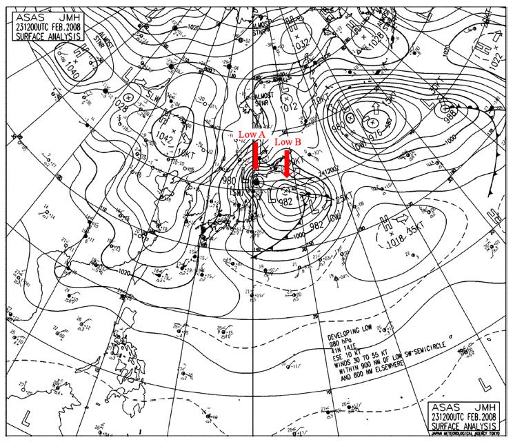
A weather chart showing the meteorological condition at 12:00 UTC 23 February 2008 is presented in Fig. 2. The Low A system generated west of Korean peninsula over the Yellow Sea at 06:00 UTC 22 February moved rapidly eastward at 12:00 UTC on the same day. Afterward, it continued to move eastward slowly over the ES, strengthening in central pressure from 1008 hPa to 992 hPa within 12 hrs. For a day from 00:00 UTC 23 to 00:00 UTC 24 February, the Low A system stayed near Hokkaido and strengthened further. Another Low B system was also developed southeast of Honshu and moved northeastward until it neared the other low system. Due to these meteorological conditions, westerly and northwesterly winds were dominant during the slow movement of the Low A over the ES on 22 February, while strong north and northeasterly winds of about 20 m/s were blowing dominantly on 23 and 24 February (Fig. 3(a)).
The observed wave characteristics from Korea Hydraulic and Oceanographic Administration (KHOA) in Korea and Nationwide Ocean Wave information network for Port and HAbourS (NOWPHAS), in Japan are presented in Table 1. From the observed wave characteristics and winds, it is found that the coastal damages around the Toyama Bay are caused by storm-induced swells (Lee et al., 2010).
2.1.2 Extreme Meteorological Conditions
In order to estimate the potential extreme storm waves in the Toyama Bay, we investigate the two factors affecting the wind wave growth, such as wind intensity and duration, by statistical analysis. The other factor, fetch, is not considered in the analysis since the observed swell directions is NNE dominant in the Toyama Bay with the fetch more than 1,000 km long.
2.1.2.1 Wind Duration
In the work of Tsuchiya et al. (1991), the following extreme value analysis (EVA) was performed for the high storm waves in the ES:
a) Observed wave characteristics over 4 m at four sites along the Japan coast facing the ES are collected from October to March for 10 yrs from 1980 to 1989.
b) The related data of the track, transition time, and central pressure from the responsible corresponding lows are also collected based on weather charts.
c) Then, apply the collected transition time data to EVA by fitting to the Gumbel distribution.
Table 2 exhibits the result of EVA in terms of transition time, which is related with and proportional to the wind duration induced by a moving low. In the following numerical experiments, the result is referred in the experiment scenarios.
2.1.2.2 Wind Intensity
In terms of extreme wind intensity condition, we compare the two events between the low in February 2008 and the one in April 2012, because the low in April 2012 is the most intensified one ever observed in extratropical cyclones in the ES. The analysis is conducted as follows:
a) Calculate the average increment rate of wind speeds due to the low in 2012 compared to those by the low in 2008. The wind speeds used are obtained from 20 AMEDAS stations from Japan Meteorological Agency (JMA) which observed the highest winds during the passage of the lows
b) Calculate the average increment rate of wind speeds based on the empirical formula for wind-pressure relationship. The minimum pressure observed in 24 February 2008 is 980 hPa, while it is 962 hPa in 3 April 2012. The difference of minimum pressure between the two events is 18 hPa. According to Knaff and Zehr (2007), the wind speed by the low in February 2008 can be intensified further about 20 m/s following the empirical formula of wind-pressure relation in case the low in February 2008 get further intensified down to 962 hPa.
c) Then, we choose the lower increment rate (160%) of wind speed between the two results obtained above for the following numerical experiments.
2.1.3 Numerical Models and Their Configurations
The atmosphere-wave modeling system consists of the following components: the Advanced Research Weather Research and Forecasting (WRF) model (v 3.2) (Skamarock et al., 2008) for the atmosphere, the third generation wind-wave model WAVEWATCH III (WW3) v 3.14 (Tolman, 2009) for the waves.
The WRF is a 3D non-hydrostatic mesoscale model developed at National Center for Atmospheric Research (NCAR) based on non-hydrostatic, compressible form of governing equations in spherical and sigma coordinates with physical processes such as precipitation physics, planetary boundary layer (PBL) processes and atmospheric radiation processes incorporated by a number of physics parameterizations. The present study adopts an interactive grid nesting with three domains with horizontal resolutions of 27, 9 and 3 km, respectively. The WRF computation is carried out for 120 hrs from 00:00 UTC 22 February to 00:00 UTC 27 February 2008. The model topography for the chosen domain regions is obtained from the U.S. Geological Survey (USGS) topography database. A Four-Dimensional Data Assimilation (FDDA) technique is also applied to all of the domains in the wind, temperature and mixing ratio fields every six hours.
The WW3 (v 3.14) is a full-spectral third-generation wind wave model developed at the Marine Modeling and Analysis Branch (MMAB) of the Environmental Modeling Center (EMC) of the National Centers for Environmental Prediction (NCEP) and freely available from NCEP. The WW3 model is applied to the storm wave simulations for the same periods with the same configuration of three nesting domains as the WRF simulation to account for the accurate swell propagation. The bathymetry for the wave simulations is taken from the GEBCO 30 arc-sec database. The external forcing is imposed from the simulated winds from the WRF model. In the last version (v3.14) of the energy balance equation of WW3 used in this study, the depth-induced wave energy dissipation term (Battjes and Janssen, 1978) is incorporated for the wave propagation in shallow water environment, which is the same formula adapted in the Simulating Waves Nearshore (SWAN) model (Booij et al., 2004). Therefore, the shallow water dynamics in the surf zone are expressed properly. In WW3, three package-like wind input and dissipation terms are available as follows: (1) The input-dissipation source terms of WAM cycle 3, which is based on Snyder et al. (1981) and Komen et al. (1984), (2) The input-dissipation package by Tolman and Chalikov (1996), which is based on Chalikov and Belevich (1993) and Chalikov (1995) for wind input and on Tolman and Chalikov (1996) for low- and high-frequency dissipation consitutents, (3) The input-dissipation source terms based on the modified wave growth theory (Janssen, 1991) and the WAM4-type dissipation term with combination of a saturation-based term (Bidlot et al., 2005).
Based on the numerical experiments of Lee (2013b) for evaluating the WW3 performance in terms of wind input and dissipation source terms, the WAM4-type input-dissipation package shows the best performance for the high storm waves in October 2005 and October 2006. Therefore, the WAM4-type wind input and whitecapping dissipation terms are used together with the discrete interaction approximation nonlinear wave-wave interactions (Hasselmann et al., 1985). The frequency increment factor (Xω), the first frequency (ω0), the number of frequencies and the directions for all of the simulations are set as 1.1, 0.04118 Hz, 25 and 36, respectively. The initial and boundary conditions for domains 2 and 3 are imposed from the mother domains, while the zero start (with the initial spectral densities of 0) is applied for domain 1 in the WW3 simulations.
2.1.4 Numerical Experiments
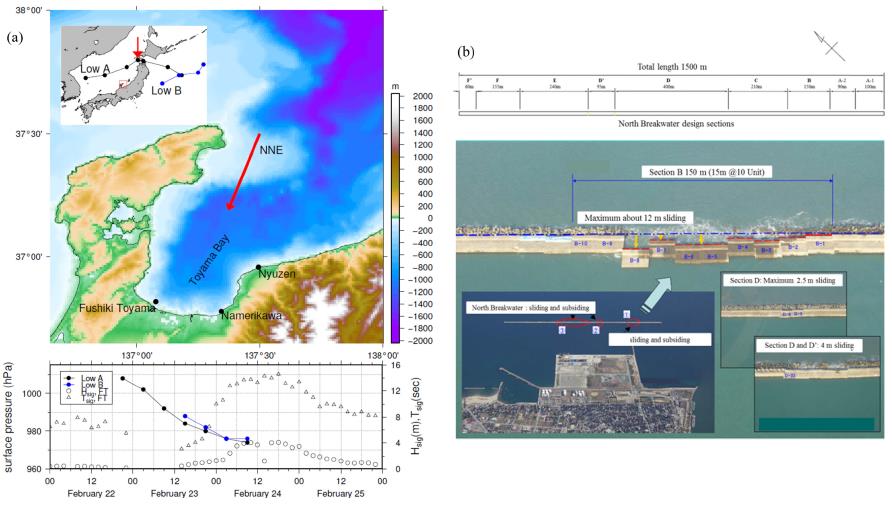
Table 3 represents the scenarios of numerical experiments conducted for estimating the extreme storm waves, Yorimawari Waves, in the Toyama Bay. Based on the extreme conditions on wind intensity and duration, five numerical experiments for wave modeling are conducted with different external forcings for wind intensities and durations. With respect to the wind duration, it is extended 6, 12 and 18 hrs from the real condition of which the low pressure stagnated near Hokkaido. For wind intensity, two conditions are considered with real and 1.6 times intensified winds. The downward red arrow in the sub-plot of the upper panel in Fig. 3(a) indicates the location of the low for the extension of wind duration.
Fig. 3.
(a) Tracks of low pressures and observed wave direction (upper panel) and the pressure variations of lows in time together with observed Hs and Ts at the Fushiki-Toyama buoy (lower panel) and (b) aerial images of the Fushiki Port and the damaged North-Breakwater (Source image from Technical Committee Report (2010)).
2.2 Part 2: Wave-Structure Interaction
2.2.1 The Fushiki Port and Damage Pattern
The Fushiki Port is located near the Fushiki-Toyama Buoy site with the 1,500 m long North-Breakwater perpendicular to the NNE direction (Fig. 3(a)). During the storm wave events in February 24 2008, the wave energies are focused on Sections B, D and D’ of the breakwater due to the refraction of waves by local bathymetry. Therefore, the corresponding sections of the breakwater are damaged with maximum 12 m, 2.5 m, and 4 m sliding backward to the pier and the armor blocks in front of the breakwater are subsided and collapsed by the storm waves (Fig. 3(b)). The storm waves of about 4 m are consistently propagated to the port more than 12 hrs.
2.2.2 Gerris flow solver (Gfs)
Gfs is an open source computational fluid dynamic code solving the non-linear shallow water equations. In this section, Gfs is described briefly in terms of the governing equations with other features. Full details of Gfs and its applications to real tsunami events and laboratory benchmark tests are referred to Popinet (2003; 2011; 2012).
The non-linear shallow water equations in conservative form with source and sink terms for Coriolis Effect and bottom friction can be described as
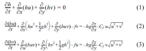
where h is free surface elevation, u = (u, v) is the horizontal velocity vector, g is the acceleration due to gravity, z is the depth of bathymetry, f is the Coriolis coefficient, and Cf is the bottom friction coefficient set to 10−3 . Additional term such as viscosity can also be added in the right hand sides of Eqs. (2)~(3) while the fundamental structure of the equations is not changed.
The non-linear shallow water equation solver used in Gfs is based on the numerical scheme analysed in detail by Audusse et al. (2004) which verifies both properties: the solver needs to properly account for vanishing fluid depths and needs to verify exactly the lake-at-rest equilibrium solution. The scheme uses a second-order, slope-limited Godunov discretization. The Riemann problem necessary to obtain Godunov fluxes is solved using an approximate Harten-Lax-van Leer Contact (HLLC) solver which guarantees positivity of the water depth. The choice of slope limiter is important as it controls the amount of numerical dissipation required to stabilize the solution close to discontinuities. Following Popinet (2011), the Sweby limiter is a good comprise between stability of short waves and low dissipation of long waves. A MUSCL-type discretization is used to generalize the method to second-order timestepping. The time-step is constrained by the Courant-Friedrich-Levy condition for stability as
where Δ‚ is the mesh size.
To summarize, the overall scheme is second-order accurate in space and time, preserves the positivity of the water depth and the lake-at-rest condition and is volume- and momentum-conserving.
Gfs uses a quadtree spatial discretization which allows efficient adaptive mesh refinement. In order to refine or coarsen the mesh dynamically, one needs to choose a refinement criterion. This choice is not trivial and depends on both the details of the numerical scheme which control how discretization errors and the physics of the problem considered which control how discretization errors will influence the accuracy of the solution. Gfs provides a variety of refinement criteria which can be flexibly combined depending on the problem. In this study, the gradient of free surface elevation was used for the refinement criterion.
2.2.3 Numerical experiments
Numerical experiments are carried out with three different configurations of the North-Breakwater to investigate its functionality against the extreme storm waves. Fig. 4 shows the computational domain in meter (2,500 m × 1,500 m) and the ambient bathymetry of the Fushiki Port. The ambient bathymetry is taken from the M7000 Digital Bathymetric Chart by Japan Hydraulic Association with reference to nearly lowest low water level. Then, the ambient bathymetry is converted to datum level with respect to Tokyo Peil (T.P.). The elevation for pier, breakwater and seawalls are taken from the 5-m resolution DEM by Geospatial Information Authority of Japan. The elevation data is referred to T.P., which is 0.15 m lower than the mean sea level of Toyama Bay.
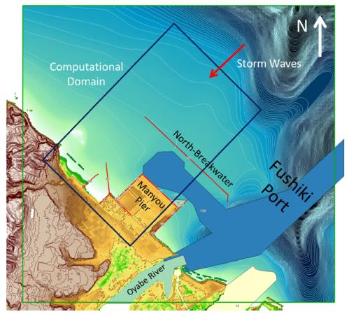
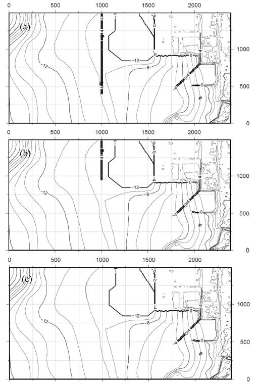
In front of the breakwater, the bathymetry changes rapidly and the water depth between the North-Breakwater and the Manyou Pier is dredged for navigational and shipping purpose. The dredged channel is extended to the mouth of the Oyabe River. Fig. 5 illustrates the three configurations of the breakwater with water depth: (a) the current condition with full functionality (CB), (b) a damaged condition with partial functionality (DB), (c) no-breakwater condition with no functionality (NoB). Table 4 also displays the details of the breakwater configurations for the experiments.
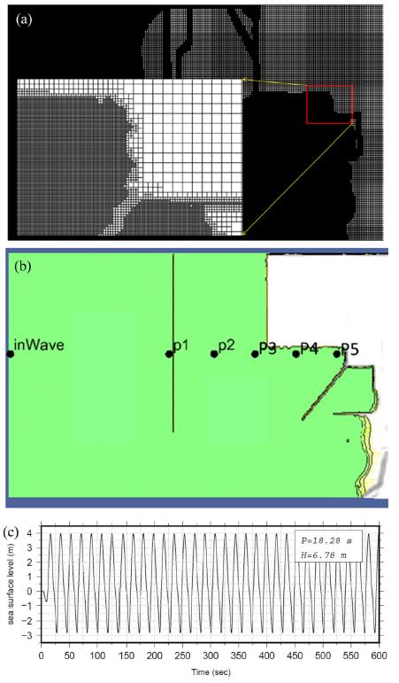
In Fig. 6(a), the initial mesh is presented illustrating the different levels of meshes depending on the local bathymetry and topography. Within the computational domain, six probes are defined to investigate the flow characteristics as illustrated in Fig. 6(b). The first probe is located just after the incident wave inputs, the second one is positioned just before the North-Breakwater, and the followings are positioned in line from left to right with the last probe placed just before the seawall in front of triangle focusing point. The incident wave profile is also displayed in Fig. 6(c) with wave height of 6.78 m and wave period of 18.28 sec in the perpendicular direction to the North-Breakwater. The two lateral sides are applied to a radiation boundary condition letting the waves freely out.
3. Results
3.1 Extreme Storm Waves
Fig. 7 exhibits the simulated wind and pressure fields using WRF and the corresponding surface wave fields with WW3 from the experiment run A. The wind fields show northerly winds clearly when the low stagnated near the Hokkaido persistently blowing for almost 24 hrs. The corresponding surface waves illustrate high wind waves over 10 m propagating from north to south. The highest wave group is focused on the northwest of the Toyama Bay. The Sado Island experiences the high waves directly and large coastal damages are occurred. The swell-like waves propagate into the Toyama Bay in NNE direction as observed.
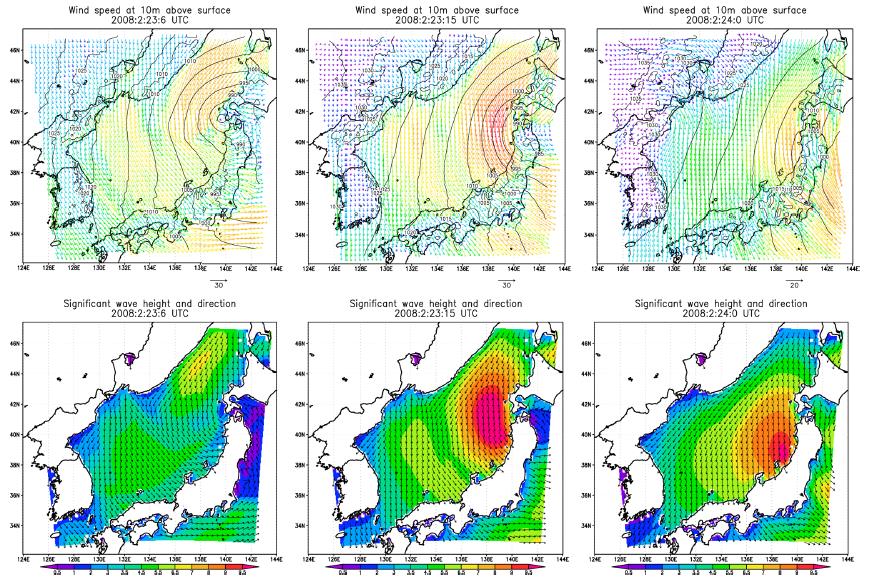
Fig. 8 illustrate the comparisons of wave characteristics between the observed and the computed from the experiment runs A to E, respectively. The hindcast result in Fig. 8(a) displays slight underestimations both in significant wave height and period. Before the storm waves are propagated into the Toyama Bay at 12:00 UTC 23 February, there seems to be long period waves with small wave heights which is not correctly simulated. Long term spin-up simulation can partly improve the results. The effects of geographical feature of the Toyama Bay such as the bay-scale resonance and coastally trapped waves can also explain the discrepancy between the observed and the computed wave characteristics.
Fig. 8(b) exhibits the comparison of wave characteristics between the observed and the computed. The computed results are from the experiment run B being forced by 1.6 times intensified winds with real duration. Both significant wave height and period are largely increased reaching up to nearly 7 m and 17 sec, respectively.
Fig. 8(c) illustrates the same comparison as in Fig. 8(a), but the computed results are from the experiment run C which uses the external wind forcing enhanced 1.6 times in wind intensity and extended 6 hrs in wind duration. The maximum significant wave height during the simulation period is nearly 7 m and the wave period is nearly 18 sec. As expected from the forcing wind duration, the high storm waves remained longer in the bay.
Fig. 8(d) represents the comparison as in Fig. 8(a), but the computed results are from the experiment run D. The external wind forcing for run D is same with run C in wind intensity, but the wind duration is extended 6 hrs more from run C. The maximum significant wave height and period are almost same with the run C, but they remained longer in the bay as expected.
Fig. 8.
Comparison of the observed and the computed significant wave heights and periods at Fushiki Toyama. The computed results are from (a) the experiment run A, (b) the experiment run B, (c) the experiment run C, (d) the experiment run D and (e) the experiment run E as in Table 3.
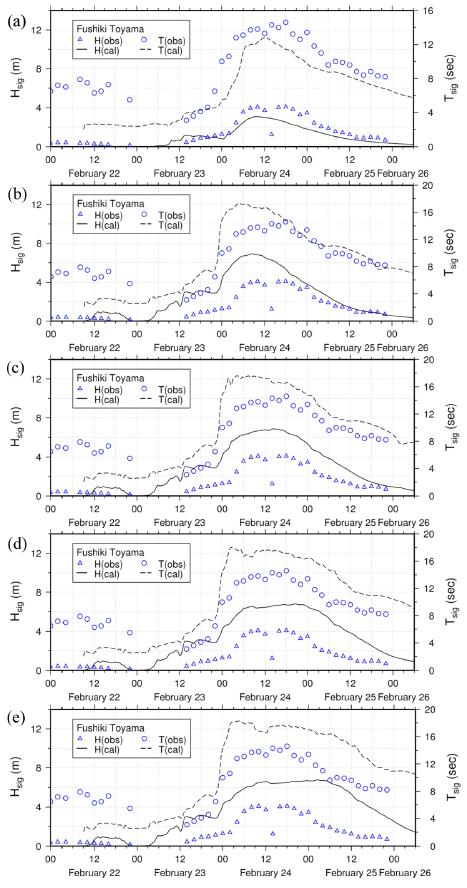
The computed results of wave characteristics from the final experiment run E are compared with the observed in Fig. 8(e). The computed maximum significant wave height is nearly 7 m and wave period is now over 18 sec. The high storm waves over 6 m is now propagating into the bay more than 24 hrs reaching to the Fushiki-Toyama site.
From the all experiment runs, the computed maximum significant wave height and period are 6.78 m and 18.28 sec at the Fushiki-Toyama buoy site.
3.2 Wave-Structure Interaction
Fig. 9 shows the sea level variations in time from the three experiments at Probe 5. Firstly, the role of the North-Breakwater can be found at the arrival time of the first wave. With the current North-Breakwater, the first wave arrives after 200 sec, while, in other results, the first waves appear before 200 sec.
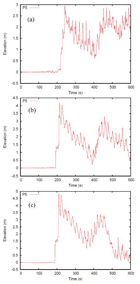
In the CB experiment’s result, the maximum water level appears to be less than 3 m by the first arrival. Then, the water level decreases gradually down to the minimum value at about 400 sec exhibiting the water level modulation due to the interaction of incoming and reflected waves between the maximum and minimum water levels. Then, the second and third peaks of water level appear at about 460 and 600 sec in the CB run. In the DB experiment, the first wave arrives just before 200 sec and the maximum water level increases over 4 m. The minimum water level within the result appears before 400 sec earlier than the CB result. Interestingly, after the second peak at about 450 sec, water level modulation becomes larger than the modulation between the maximum and minimum water levels from 200 to 400 sec. In the NoB results, the first wave arrives slightly earlier than the DB case and the maximum water level reaches nearly 5 m before 200 sec. The minimum water level is also presented earlier that the other runs at about 360 sec with about 1 m, which is the highest value among the experiments. Noticeably, after the second peak at about 440 sec, the water level depicts smooth drops compared to the other runs, resulting from the large overtopping of waves.
Fig. 10 to 12 illustrate the 3D snapshots of sea level variations. In the CB results of Fig. 10, the role of the North-Breakwater is clearly presented that the front of Manyou Pier is not overtopped due to the North-Breakwater. However, the Manyou Pier is overtopped from the side-seawall where the Probe 4 and 5 are positioned. Since the height of side-seawall of the Manyou Pier is gradually decreasing, the side-seawall overtopping is visible after 300 sec. In addition, the heavy overtopping in the inner Manyou Pier is outstanding from the side-seawall next to the small port formed by the oblique breakwater in the left of Probe 5 and groyne. One of the outstanding features by using the adaptive mesh is the small vortices formed by diffraction and interactions of waves near the edge of breakwaters. However, since the non-linear shallow water equations do not include the viscous term, the vortices keep their motions without turbulent and viscous dissipations.
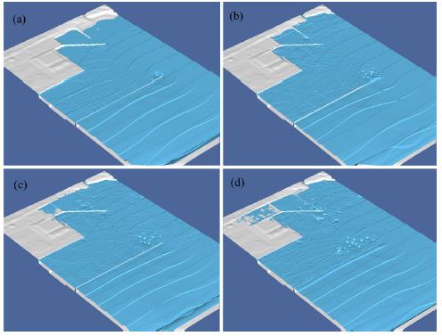
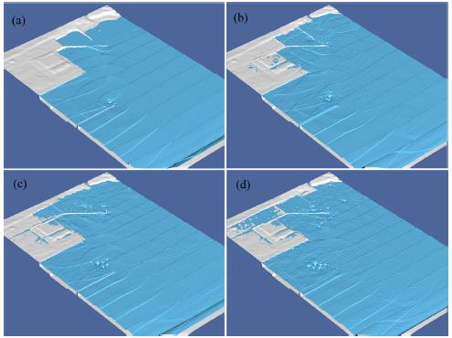
The wet-dry scheme together with adaptive meshes is able to model the run-up and capture the shoreline changes well and efficiently depending on flow features, which is the free surface gradient in this study.
Fig. 11 exhibits the 3D snapshot of sea level variations from the DB run, which considers the partial damage of the North-Breakwater. It is illustrated at the snapshot at 180 sec that the first wave arrives faster than the CB run. The overtopping from the side-seawall occurs earlier in time and larger in volume than the CB run. Also the overtopping over the side-seawall from the small port becomes severer and the inner Manyou Pier is heavily flooded. Small vortices are also observed in the DB results. An overtopping over the front seawall is not observed in the DB run.
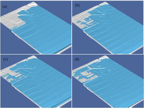
Fig. 12 represents the 3D snapshots from the no breakwater case, the NoB run, at 180, 300, 420 and 540 sec after the simulation starts. The first wave arrival is depicted at the 180-sec snapshot and the front seawall of the Manyou Pier is visible at this time step. The Manyou Pier experiences complete flooding from the front and side seawall. The small port next to the inner Manyou Pier is totally packed with sea water. A number of small vortices are also observed near the oblique breakwater.
4. Discussions
In order to estimate extreme wave characteristics, there are two ways in general:
a) Apply the long-term observed wave characteristics to EVA to find out the extreme storm wave characteristics for a target return period.
b) Find out the extreme conditions for wind intensity and duration for given fetch, and then conduct numerical experiments for wind waves with the extreme conditions for wind forcing.
In the present study, we investigate the extreme wave characteristics by examining the extreme conditions for wind intensity and duration for the event of February 2008. It could be possible, however, to combine the method a) and b) together. First, investigate the probabilities of extreme wind forcings in terms of wind intensity and duration. Then, conduct wind wave modelings with the given extreme meteorological conditions. Finally, apply the resulting wave characteristics to EVA to obtain the extreme storm wave characteristics. The combined method might be more physics-based statistical approach by combining meteorological and wave modeling, and statistical modeling.
Unlike the Best track data for tropical cyclones, there is no such historical data archive for the track and central pressure of low pressures (e.g. extratropical cyclones) responsible for the high storm waves in the winter ES. To perform the statistical analysis for wind intensity and duration described above, such historical data archive is necessary and have to be established.
As demonstrated in the event of April 2012, the increased supply of latent heat and water vapor could intensify a moving low unprecedentedly rapid. It is mainly due to the extension of the Tsushima Warm Currents. In the future climate, it is feasible that the warmer ocean environment could impact the overlying meteorological conditions, then back to the surface waves. Such potential impacts of climate changes have to be also taken into account for a study of extreme storm waves in the ES.
5. Conclusions
In the winter East Sea, coastal damages and disasters in Korean and Japanese coasts are often occurred by storm waves due to rapidly developing low pressure systems. In February 2008, storm waves due to a moving low propagating from the west off Hokkaido, Japan, to the south and southwest caused severe coastal damages along the Toyama Bay coast. In particular, the Fushiki Port in the Toyama Bay experienced severe damage in its North-Breakwater which protects the Manyou Pier behind in the south.
Therefore, in the first part of the study, we investigate the extreme storm waves in the Toyama Bay, Japan, by examining the extreme conditions for wind intensity and duration for the event of February 2008. The wind fetch is more or less pre-determined, therefore it is not considered in the analysis.
In terms of wind intensity, we compare the observed wind speeds due to the lows in February 2008 and in April 2012 to obtain an extreme condition, because the low in April 2012 breaks the records in observed winds and central pressure in its kind of winter storms (e.g. extratropical cyclones). With respect to the wind duration, a statistical analysis result for transition time of lows passing over the ES is used to find out the extreme conditions for wind duration.
For the given extreme conditions for wind intensity and duration, numerical experiments are carried out to estimate the extreme storm waves in the Toyama Bay. The resulting significant wave height and period at the Fushiki-Toyama buoy site in the Toyama Bay are 6.78 m and 18.28 sec, respectively.
To improve the extreme storm wave estimation, we discuss and suggest the possible approaches by combining deterministic and statistical methods. Further, the impacts of future warming climate on meteorological conditions and back on surface waves have to be addressed in future works.
In the second part, we investigate the functionality of the North-Breakwater in the Fushiki Port, Toyama Bay against the estimated extreme storm waves with Hs of 6.78 m and Ts of 18.28 sec used for the incident wave profile.
Numerical experiments using a non-linear shallow water equation model with adaptive mesh refinement method are carried out to investigate the North-Breakwater functionality. Three experiments are considered for current, damaged and no breakwater cases. In all runs, the inner Manyou Pier becomes overtopped over the side seawall adjacent to a small port formed by breakwater and groyne. The North-Breakwater is proved to be a protector for the Manyou Pier from overtopping over the front seawall. It also affects the maximum water level and arrival time of the first wave.
In this numerical experiment, however, there are a couple of limitations as follows. Firstly, the functionality of the North-Breakwater is not directly and explicitly considered in the simulation. Therefore, it is unknown that if the North-Breakwater itself would be damaged, for example, sliding or overturning due to the extreme storm waves. Secondly, the temporal profile of the incident waves at the open boundary does represent a series of sinusoidal waves with wave height of 6.78 m and wave period of 18.28 sec rather than representing wave characteristics of irregular waves with Hs and Ts.
Therefore, those limitations have to be considered when interpreting the simulation results of this study and have to be improved in further works.


